Franck-Condon Principle
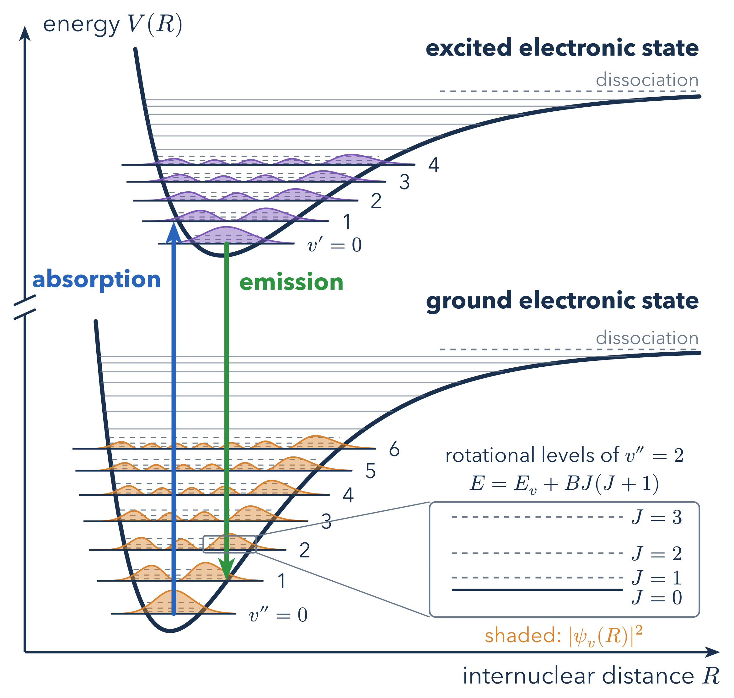
Potential energy curves of a diatomic molecule in its ground and first excited electronic states, drawn as Morse potentials with exact vibrational levels that crowd together toward the dissociation limit. Each shaded curve is the vibrational probability density resting on its level, and dashed lines mark the rotational sublevels , enlarged in the inset for .
Electrons move much faster than nuclei, so an electronic transition happens at fixed internuclear distance : absorption and emission are vertical arrows. Their intensities follow the Franck-Condon factors , the squared overlaps of the two vibrational wavefunctions. Because the excited state has a longer, softer bond, absorption from lands most likely in and emission from in ; both arrows end on the level with the largest overlap computed from the plotted wavefunctions. Emission thus has lower energy than absorption (the Stokes shift), and the spread of Franck-Condon factors produces the vibrational progressions seen in molecular spectra.
Download
Code
#import "@preview/cetz:0.5.3": canvas, draw
#import draw: content, line, rect

// Ground and excited electronic states as Morse potentials V(R) = T_e + D (1 - e^(-a (R - R_e)))^2
// with exact Morse levels and wavefunctions (equal reduced masses). Arrows end on the level with
// the largest Franck-Condon factor |<v'|v''>|^2, from the wavefunction overlaps computed below.
// https://doi.org/10.1103/PhysRev.34.57 https://doi.org/10.1039/TF9262100536
#set page(width: auto, height: auto, margin: 8pt, fill: none)
#let (ink, muted, orange) = ("#19304E", "#6A788B", "#D9822B").map(rgb)
#let (purple, blue, green) = ("#7B57B8", "#2864BB", "#2E9440").map(rgb)
#set text(font: "Avenir Next", size: 14pt, fill: ink)

// lambda = sqrt(2 m D) / (a hbar), so equal masses scale it with sqrt(D) / a
#let ground = (D: 6, a: 1.0, Re: 3.0, lam: 16, Te: 0, B: 0.02, n: 7)
#let excited = (D: 3.5, a: 0.9, Re: 3.5, Te: 8, B: 0.015, n: 5)
#let excited = excited + (lam: ground.lam * calc.sqrt(excited.D / ground.D) * ground.a / excited.a)
#assert(
  ground.n < ground.lam - 0.5 and excited.n < excited.lam - 0.5,
  message: "n exceeds bound levels",
)
#let V(s, R) = s.Te + s.D * calc.pow(1 - calc.exp(-s.a * (R - s.Re)), 2)
#let level(s, v) = s.Te + s.D * (1 - calc.pow(1 - (v + 0.5) / s.lam, 2))
// Classical turning point at energy E: inner (sign 1) or outer (sign -1)
#let turning(s, E, sign: 1) = s.Re - calc.ln(1 + sign * calc.sqrt((E - s.Te) / s.D)) / s.a

// Morse eigenfunctions z^s e^(-z/2) L_v^(2s)(z) for z = 2 lambda e^(-a (R - R_e)) and
// s = lambda - v - 1/2, with Laguerre polynomials L by upward recurrence, normalized on the grid
#let (R-min, dR) = (1.0, 11 / 1600)
#let grid = range(1601).map(idx => R-min + idx * dR)
#let laguerre(n, alpha, z) = {
  let (p, c) = (1.0, 1.0 + alpha - z)
  for k in range(1, n) { (p, c) = (c, ((2 * k + 1 + alpha - z) * c - (k + alpha) * p) / (k + 1)) }
  if n == 0 { p } else { c }
}
#let morse-psi(s, v) = {
  let sv = s.lam - v - 0.5
  let zs = grid.map(R => 2 * s.lam * calc.exp(-s.a * (R - s.Re)))
  let vals = zs.map(z => calc.exp(sv * calc.ln(z) - z / 2) * laguerre(v, 2 * sv, z))
  let total = calc.sqrt(vals.map(x => x * x).sum() * dR)
  vals.map(x => x / total)
}
#let (ground, excited) = (ground, excited).map(s => s + (psi: range(s.n).map(v => morse-psi(s, v))))
#let argmax(xs) = xs.position(x => x == calc.max(..xs))
// Vertical transition from v = 0 at its most probable R to the level with the largest overlap
#let transition(s0, s1) = {
  let to = argmax(s1.psi.map(p => calc.pow(p.zip(s0.psi.at(0)).map(((x, y)) => x * y).sum(), 2)))
  (R: grid.at(argmax(s0.psi.at(0).map(x => x * x))), E0: level(s0, 0), E1: level(s1, to), to: to)
}
#let (absorb, emit) = (transition(ground, excited), transition(excited, ground))
#assert.eq((absorb.to, emit.to), (1, 1))

#let R-end = 8.1 // plotted R from 1.6 to R-end
#let P(R, E) = (2.1 * (R - 1.6), 0.95 * E)

#let vib-levels(s, color, prime, height) = for v in range(calc.ceil(s.lam - 0.5)) {
  let (E, peak) = (level(s, v), calc.max(..s.psi.at(0).map(x => x * x)))
  let (R-left, R-right) = (turning(s, E), turning(s, E, sign: -1))
  if v >= s.n {
    // weakly bound levels crowding toward the dissociation limit (within the plotted R)
    if R-right <= R-end {
      line(P(R-left, E), P(R-right, E), stroke: muted.transparentize(30%) + 0.6pt)
    }
    continue
  }
  // rotational sublevels J = 1, 2, 3, then |psi_v(R)|^2 resting on the level
  for E-J in (1, 2, 3).map(J => E + s.B * J * (J + 1)) {
    line(P(R-left, E-J), P(R-right, E-J), stroke: (paint: muted, thickness: 0.6pt, dash: "dashed"))
  }
  let (R0, R1) = (R-left - 0.35, R-right + 0.35)
  let density = grid.zip(s.psi.at(v)).filter(((R, _)) => R0 <= R and R <= R1)
  let pts = density.map(((R, p)) => P(R, E + height * p * p / peak))
  line(P(R0, E), ..pts, P(R1, E), fill: color.transparentize(55%), stroke: color + 0.9pt)
  line(P(R0, E), P(R1, E), stroke: ink + 1pt)
  let label = if v == 0 { $v#prime = 0$ } else { str(v) }
  content(P(R1 + 0.12, E), text(12pt, label), anchor: "west")
}

#canvas(length: 1cm, {
  // Energy axis with a break between the electronic states, internuclear-distance axis
  let axis = (stroke: ink + 1.4pt, mark: (end: "stealth", fill: ink, scale: 0.9))
  line(P(1.6, -0.45), P(1.6, 6.75), stroke: ink + 1.4pt)
  line(P(1.6, 7.05), P(1.6, 12.9), ..axis)
  for E in (6.75, 7.05) {
    line((-0.22, 0.95 * E - 0.1), (0.22, 0.95 * E + 0.1), stroke: ink + 1.4pt)
  }
  line(P(1.6, -0.45), P(R-end + 0.2, -0.45), ..axis)
  content(P(R-end + 0.2, -0.75), [internuclear distance $R$], anchor: "north-east")
  content(P(1.77, 12.9), [energy $V(R)$], anchor: "west")

  // Potentials from where the repulsive wall reaches E-top, dissociation limits and labels
  for (s, E-top, label) in ((ground, 6.6, [ground]), (excited, 12.4, [excited])) {
    let curve = range(201).map(idx => turning(s, E-top) + (R-end - turning(s, E-top)) * idx / 200)
    line(..curve.map(R => P(R, V(s, R))), stroke: (paint: ink, thickness: 2.4pt, cap: "round"))
    let y = s.Te + s.D
    line(P(5.6, y), P(R-end, y), stroke: (paint: muted, thickness: 0.9pt, dash: "dashed"))
    content(P(R-end, y + 0.11), text(11pt, fill: muted)[dissociation], anchor: "south-east")
    content(P(R-end, y + 0.75), strong[#label electronic state], anchor: "south-east")
  }
  vib-levels(ground, orange, $''$, 0.5)
  vib-levels(excited, purple, $'$, 0.36)

  // Franck-Condon transitions: vertical at fixed R
  for (t, color, label) in ((absorb, blue, [absorption]), (emit, green, [emission])) {
    let (stroke, tip) = ((paint: color, thickness: 2.6pt, cap: "round"), (fill: color, scale: 1.1))
    line(P(t.R, t.E0), P(t.R, t.E1), stroke: stroke, mark: tip + (end: "stealth"))
    let (dx, anchor) = if t == absorb { (-0.12, "east") } else { (0.12, "west") }
    content(P(t.R + dx, 7.45), text(fill: color, weight: "bold", label), anchor: anchor)
  }

  // Zoom on the rotational sublevels of v'' = 2
  let (E2, R2) = (level(ground, 2), turning(ground, level(ground, 2), sign: -1))
  let (zoom-lo, zoom-hi) = (P(R2 - 0.45, E2 - 0.06), P(R2 + 0.06, E2 + 12 * ground.B + 0.06))
  let (lo, hi) = (P(5.5, 0.3), P(R-end, 2.75))
  rect(zoom-lo, zoom-hi, stroke: muted + 0.9pt, radius: 0.04)
  line(zoom-hi, (lo.at(0), hi.at(1)), stroke: muted + 0.7pt)
  line((zoom-hi.at(0), zoom-lo.at(1)), lo, stroke: muted + 0.7pt)
  rect(lo, hi, stroke: muted + 0.9pt, fill: white, radius: 0.12)
  let (x0, x1, y0, y1) = (lo.at(0) + 0.45, hi.at(0) - 1.55, lo.at(1) + 0.55, hi.at(1) - 0.3)
  let dashed = (paint: muted, thickness: 1pt, dash: "dashed")
  for J in range(4) {
    let y = y0 + (y1 - y0) * J * (J + 1) / 12
    // J = 0 and 1 lie close together, so the J = 0 label sits below its line
    let (stroke, anchor) = if J == 0 { (ink + 1.2pt, "north-west") } else { (dashed, "west") }
    line((x0, y), (x1, y), stroke: stroke)
    content((x1 + 0.15, y), text(12pt)[$J = #J$], anchor: anchor)
  }
  let cx = (lo.at(0) + hi.at(0)) / 2
  let title = text(12pt, align(center)[rotational levels of $v'' = 2$ \ $E = E_v + B J(J + 1)$])
  content((cx, hi.at(1) + 0.14), title, anchor: "south")
  content((cx, lo.at(1) - 0.21), text(12pt, fill: orange)[shaded: $|psi_v (R)|^2$], anchor: "north")
})