GW Approximation
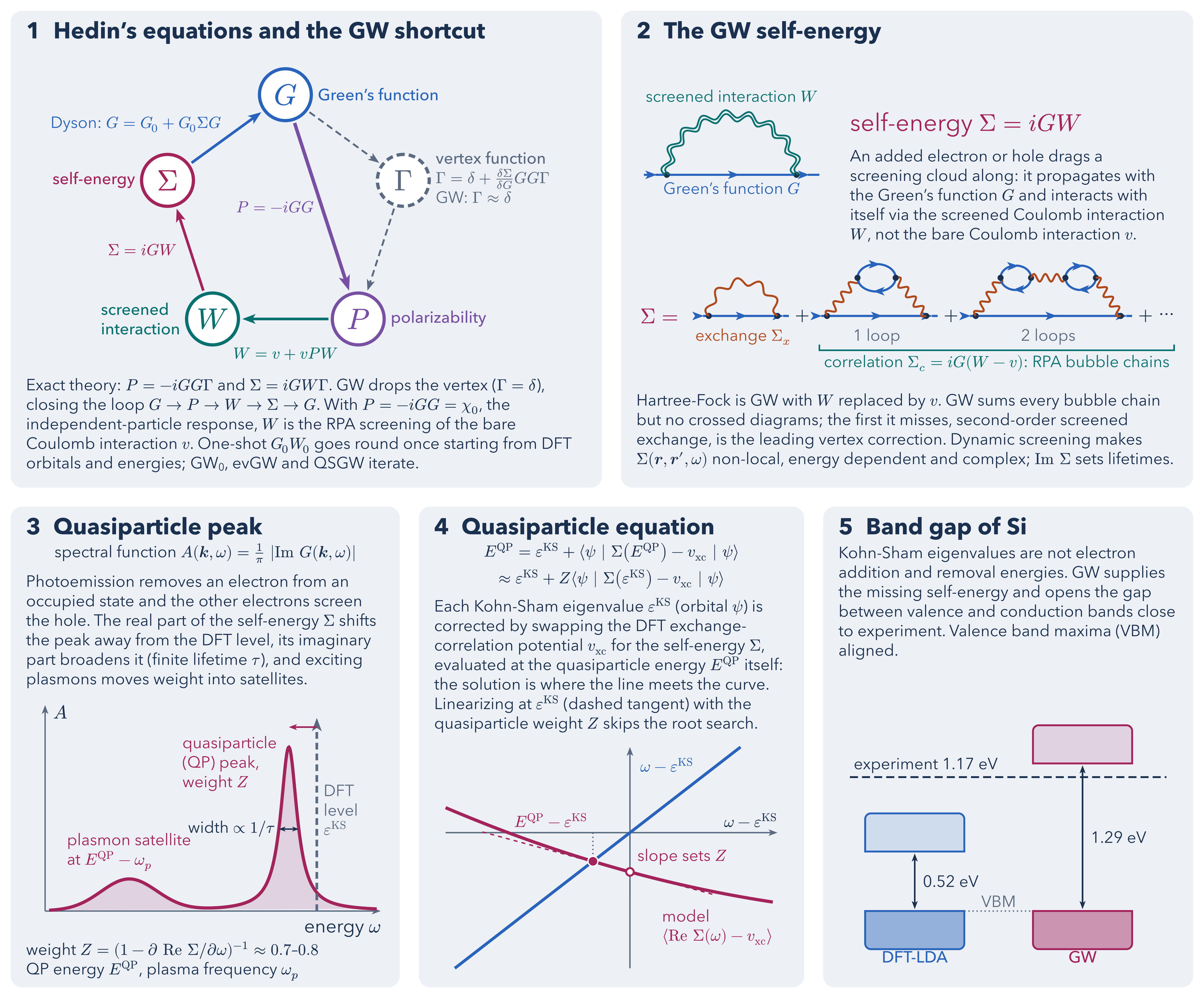
The GW approximation for quasiparticle energies in five panels. (1) Hedin's equations link the Green's function , polarizability , screened interaction , self-energy and vertex in a closed pentagon. GW sets , which short-circuits the vertex and leaves the loop through Dyson's equation. With , is exactly the RPA screened interaction (see the Random Phase Approximation diagram). (2) The self-energy is an electron line with a screened interaction attached at both ends. Expanding splits it into bare exchange (Hartree-Fock) and correlation from bubble chains, which makes non-local, energy dependent and complex.
(3) The spectral function replaces the sharp mean-field level with a shifted quasiparticle peak of weight and width , plus a plasmon satellite near (schematic Lorentzian and Gaussian). (4) The quasiparticle equation is solved where meets the self-energy curve (a quadratic model); linearizing at gives the usual . (5) For silicon, GW opens the indirect gap from 0.52 eV (LDA) to 1.29 eV, compared with 1.17 eV measured (Hybertsen and Louie 1986).
Download
Code
#import "@preview/cetz:0.5.3": canvas, draw
#import draw: circle, content, line, rect

// GW approximation: Hedin's pentagon with the vertex dropped, the GW self-energy and its
// exchange + correlation split, the quasiparticle spectral function, the graphical solution of
// the quasiparticle equation (model Sigma) and the Si band gap of Hybertsen and Louie (1986).
// https://doi.org/10.1103/PhysRev.139.A796 https://doi.org/10.1103/PhysRevB.34.5390
#set page(width: auto, height: auto, margin: 8pt, fill: none)
#let (ink, muted, panel-fill) = (rgb("#19304E"), rgb("#5A6A80"), rgb("#EDF1F6"))
#set text(font: "Avenir Next", size: 14pt, fill: ink)
#set par(leading: 0.5em)
// Same colors as the RPA diagram: fermions, bare v, screened W, polarization; plus Sigma
#let (c-el, c-v, c-w, c-chi, c-sig) = ("#2864BB", "#B04A1C", "#06716E", "#7750A3", "#A3245B").map(
  rgb,
)

#let small(body, ..args) = text(size: 12pt, ..args, body)
#let tip(color, scale) = (end: "stealth", fill: color, scale: scale)
#let mapper(origin, width, height, (x0, x1), (y0, y1)) = ((x, y)) => (
  origin.at(0) + (x - x0) / (x1 - x0) * width,
  origin.at(1) + (y - y0) / (y1 - y0) * height,
)
#let axes(to-canvas, (x0, x1), (y0, y1), x-label, y-label, y-axis-x: 0) = {
  line(to-canvas((x0, 0)), to-canvas((x1, 0)), stroke: muted + 1pt, mark: tip(muted, 0.7))
  line(to-canvas((y-axis-x, y0)), to-canvas((y-axis-x, y1)), stroke: muted + 1pt, mark: tip(
    muted,
    0.7,
  ))
  content(to-canvas((x1, 0)), x-label, anchor: "north-east", padding: (top: 6pt))
  content(to-canvas((y-axis-x, y1)), y-label, anchor: "north-west", padding: (left: 6pt))
}
#let samples((x0, x1), n: 200) = range(n + 1).map(idx => x0 + (x1 - x0) * idx / n)
#let panel((x0, y0), (x1, y1), title) = {
  rect((x0, y0), (x1, y1), fill: panel-fill, stroke: none, radius: 0.3)
  content((x0 + 0.4, y0 - 0.3), text(17pt, weight: "bold", title), anchor: "north-west")
}
#let note((x, y), width, body, anchor: "north-west") = content(
  (x, y),
  box(width: width * 1cm, small(body)),
  anchor: anchor,
)

// === Feynman parts on parametric curves p(t), t in [0, 1] ===
#let straight(start, end) = frac => start.zip(end).map(((from, to)) => from + (to - from) * frac)
#let arc((cx, cy), rx, ry, start, sweep) = frac => (
  cx + rx * calc.cos(start + sweep * frac),
  cy + ry * calc.sin(start + sweep * frac),
)
#let wavy(curve, waves: 4, amp: 0.1, offset: 0, color: c-v, width: 1.5pt) = line(
  ..range(waves * 16 + 1).map(idx => {
    let frac = idx / (waves * 16)
    let ((x1, y1), (x2, y2)) = (curve(calc.max(frac - 1e-3, 0)), curve(calc.min(frac + 1e-3, 1)))
    let shift = (offset + amp * calc.sin(2 * calc.pi * waves * frac)) / calc.norm(x2 - x1, y2 - y1)
    let (x, y) = curve(frac)
    (x - (y2 - y1) * shift, y + (x2 - x1) * shift)
  }),
  stroke: color + width,
)
#let n-waves(start, end) = calc.max(2, int(calc.round(
  calc.norm(..start.zip(end).map(((from, to)) => to - from)) / 0.32,
)))
#let coulomb(start, end) = wavy(straight(start, end), waves: n-waves(start, end))
#let screened(curve, waves) = for offset in (-0.05, 0.05) {
  wavy(curve, waves: waves, offset: offset, color: c-w, width: 1.3pt)
}
#let fermion(curve, color: c-el, width: 1.6pt) = {
  let pts(from, to) = range(31).map(idx => curve(from + (to - from) * idx / 30))
  line(..pts(0, 0.56), stroke: color + width, mark: tip(color, 0.75))
  line(..pts(0.5, 1), stroke: color + width)
}
#let vertex(pos) = circle(pos, radius: 0.08, fill: ink, stroke: none)
#let bubble((cx, y), rx, ry) = {
  fermion(arc((cx, y), rx, ry, 180deg, -180deg))
  fermion(arc((cx, y), rx, ry, 0deg, -180deg))
  for x in (cx - rx, cx + rx) { vertex((x, y)) }
}
// Electron line through interaction vertices at xa and xb, with external legs of length leg
#let sigma-line(xa, xb, y, leg: 0.3) = {
  for (from, to) in ((xa - leg, xa), (xa, xb), (xb, xb + leg)) {
    fermion(straight((from, y), (to, y)))
  }
  for x in (xa, xb) { vertex((x, y)) }
}

// === Spectral function: QP Lorentzian (weight Z, half width gamma) plus plasmon satellite ===
#let (e-ks, e-qp, z-qp, gamma, omega-p, sat-width) = (0, -0.7, 0.7, 0.25, 4, 0.7)
#let spectral(w) = (
  z-qp * gamma / calc.pi / (calc.pow(w - e-qp, 2) + gamma * gamma)
    + (1 - z-qp)
      * calc.exp(-calc.pow(w - e-qp + omega-p, 2) / (2 * sat-width * sat-width))
      / (sat-width * calc.sqrt(2 * calc.pi))
)

// === Model <Re Sigma(omega) - v_xc> about epsilon_KS = 0 for the QP-equation panel ===
#let (sig-0, sig-slope, sig-curv) = (-0.55, -0.35, 0.05)
#let sigma-model(x) = sig-0 + sig-slope * x + sig-curv * x * x
// Root of x = sigma-model(x) and the linearized estimate Z * sigma-model(0)
#let x-qp = (
  (1 - sig-slope - calc.sqrt(calc.pow(1 - sig-slope, 2) - 4 * sig-curv * sig-0)) / (2 * sig-curv)
)
#let z-model = 1 / (1 - sig-slope)
#assert(calc.abs(x-qp - sigma-model(x-qp)) < 1e-9 and calc.abs(x-qp - z-model * sig-0) < 0.02)

// Si indirect gap in eV, Hybertsen and Louie, PRB 34, 5390 (1986)
#let (gap-lda, gap-gw, gap-exp) = (0.52, 1.29, 1.17)

#canvas(length: 1cm, {
  // === 1: Hedin's pentagon ===
  panel((0, 0), (15.5, -12.5), [1 #h(0.3em) Hedin's equations and the GW shortcut])
  let (cx, cy, radius, node-r) = (7.2, -5.45, 3.25, 0.68)
  let names = ("G", "Gamma", "P", "W", "Sigma")
  let pos = range(5).map(idx => (
    cx + radius * calc.cos(90deg - idx * 72deg),
    cy + radius * calc.sin(90deg - idx * 72deg),
  ))
  let node = names.zip(pos).to-dict()
  let colors = (G: c-el, Gamma: muted, P: c-chi, W: c-w, Sigma: c-sig)
  let link(from, to, color, faded: false, width: 2pt) = {
    let ((x0, y0), (x1, y1)) = (node.at(from), node.at(to))
    let len = calc.norm(x1 - x0, y1 - y0)
    let gap = (node-r + 0.1) / len
    let stroke = (paint: color, thickness: width, dash: if faded { (5pt, 3pt) })
    line(
      (x0 + gap * (x1 - x0), y0 + gap * (y1 - y0)),
      (x1 - gap * (x1 - x0), y1 - gap * (y1 - y0)),
      stroke: stroke,
      mark: tip(color, 0.8),
    )
  }
  link("G", "Gamma", muted, faded: true, width: 1.4pt)
  link("Gamma", "P", muted, faded: true, width: 1.4pt)
  link("G", "P", c-chi, width: 2.6pt)
  link("P", "W", c-w)
  link("W", "Sigma", c-sig)
  link("Sigma", "G", c-el)
  for name in names {
    let color = colors.at(name)
    let faded = name == "Gamma"
    circle(node.at(name), radius: node-r, fill: white, stroke: (
      paint: color,
      thickness: 2.4pt,
      dash: if faded { (5pt, 3pt) },
    ))
    content(node.at(name), text(22pt, fill: color, math.equation(eval(name, mode: "math"))))
  }
  let node-names = (
    G: ([Green's function], "west", (left: 0.85cm)),
    Sigma: ([self-energy], "east", (right: 0.85cm)),
    W: ([screened\ interaction], "east", (right: 0.85cm)),
    P: ([polarizability], "west", (left: 0.85cm)),
  )
  for (name, (body, anchor, padding)) in node-names {
    content(
      node.at(name),
      small(fill: colors.at(name), weight: "medium", body),
      anchor: anchor,
      padding: padding,
    )
  }
  let mid(from, to) = node.at(from).zip(node.at(to)).map(((start, end)) => (start + end) / 2)
  content(
    mid("Sigma", "G"),
    small(fill: c-el)[Dyson: $G = G_0 + G_0 Sigma G$],
    anchor: "south-east",
    padding: (right: 4pt, bottom: 4pt),
  )
  content(mid("W", "Sigma"), small(fill: c-sig)[$Sigma = i G W$], anchor: "east", padding: 10pt)
  content(mid("P", "W"), small(fill: c-w)[$W = v + v P W$], anchor: "north", padding: (top: 0.75cm))
  content(mid("G", "P"), small(fill: c-chi)[$P = -i G G$], anchor: "east", padding: 6pt)
  let vertex-note = [#text(weight: "medium")[vertex function] \ $Gamma = delta + (delta Sigma) / (delta G) G G Gamma$ \ GW: $Gamma approx delta$]
  content(node.at("Gamma"), small(fill: muted, vertex-note), anchor: "west", padding: (
    left: 0.85cm,
  ))
  let hedin-note = [Exact theory: $P = -i G G Gamma$ and $Sigma = i G W Gamma$. GW drops the vertex ($Gamma = delta$), closing the loop $G -> P -> W -> Sigma -> G$. With $P = -i G G = chi_0$, the independent-particle response, $W$ is the RPA screening of the bare Coulomb interaction $v$. One-shot $G_0 W_0$ goes round once starting from DFT orbitals and energies; GW#sub[0], evGW and QSGW iterate.]
  note((0.4, -9.65), 14.7, hedin-note)

  // === 2: GW self-energy ===
  panel((16, 0), (31, -12.5), [2 #h(0.3em) The GW self-energy])
  let y = -4.3
  let (xa, xb) = (17.2, 20.6)
  sigma-line(xa, xb, y, leg: 0.6)
  screened(arc(((xa + xb) / 2, y), 1.7, 1.55, 180deg, -180deg), 9)
  content(((xa + xb) / 2, y - 0.2), small(fill: c-el)[Green's function $G$], anchor: "north")
  content(
    ((xa + xb) / 2, y + 1.8),
    small(fill: c-w)[screened interaction $W$],
    anchor: "south",
    padding: 3pt,
  )
  content((22.0, -3.0), text(18pt, fill: c-sig)[self-energy $Sigma = i G W$], anchor: "west")
  let sigma-note = [An added electron or hole drags a screening cloud along: it propagates with the Green's function $G$ and interacts with itself via the screened Coulomb interaction $W$, not the bare Coulomb interaction $v$.]
  note((22.0, -3.65), 8.6, sigma-note)
  // Expansion of W: exchange (bare v) plus correlation (bubble chains with 1, 2, ... loops)
  let y = -8
  content((16.5, y), text(16pt, fill: c-sig)[$Sigma =$], anchor: "west")
  let (xa, xb) = (18.3, 20.1)
  sigma-line(xa, xb, y)
  wavy(arc(((xa + xb) / 2, y), 0.9, 0.9, 180deg, -180deg), waves: 5)
  content(((xa + xb) / 2, y - 0.35), small(fill: c-v)[exchange $Sigma_x$], anchor: "north")
  content((20.75, y), $+$)
  let (xa, xb) = (21.4, 24)
  sigma-line(xa, xb, y)
  let (xc, top) = ((xa + xb) / 2, y + 1)
  coulomb((xa, y), (xc - 0.5, top))
  coulomb((xc + 0.5, top), (xb, y))
  bubble((xc, top), 0.5, 0.36)
  content((xc, y - 0.35), small(fill: muted)[1 loop], anchor: "north")
  content((24.65, y), $+$)
  let (xa, xb) = (25.3, 29.1)
  sigma-line(xa, xb, y)
  let xc = (xa + xb) / 2
  coulomb((xa, y), (xc - 1.25, top))
  bubble((xc - 0.85, top), 0.4, 0.32)
  coulomb((xc - 0.45, top), (xc + 0.45, top))
  bubble((xc + 0.85, top), 0.4, 0.32)
  coulomb((xc + 1.25, top), (xb, y))
  content((xc, y - 0.35), small(fill: muted)[2 loops], anchor: "north")
  content((29.75, y), $+$)
  content((30.3, y), $dots.c$)
  let (x0, x1, yb) = (21.2, 30.5, y - 0.9)
  line((x0, yb + 0.15), (x0, yb), (x1, yb), (x1, yb + 0.15), stroke: c-w + 1.2pt)
  content(
    ((x0 + x1) / 2, yb),
    small(fill: c-w)[correlation $Sigma_c = i G (W - v)$: RPA bubble chains],
    anchor: "north",
    padding: (top: 4pt),
  )
  let split-note = [Hartree-Fock is GW with $W$ replaced by $v$. GW sums every bubble chain but no crossed diagrams; the first it misses, second-order screened exchange, is the leading vertex correction. Dynamic screening makes $Sigma(bold(r), bold(r)', omega)$ non-local, energy dependent and complex; $"Im" Sigma$ sets lifetimes.]
  note((16.4, -10.05), 14.2, split-note)

  // === 3: spectral function ===
  panel((0, -13), (10.2, -25.6), [3 #h(0.3em) Quasiparticle peak])
  content(
    (5.1, -14.25),
    small[spectral function $A(bold(k), omega) = 1 / pi |"Im" G(bold(k), omega)|$],
  )
  let peak-note = [Photoemission removes an electron from an occupied state and the other electrons screen the hole. The real part of the self-energy $Sigma$ shifts the peak away from the DFT level, its imaginary part broadens it (finite lifetime $tau$), and exciting plasmons moves weight into satellites.]
  note((0.4, -14.8), 9.4, peak-note)
  let (w-lim, a-lim) = ((-6.8, 1.6), (0, 1.12))
  let to-canvas = mapper((0.9, -23.6), 8.8, 5.4, w-lim, a-lim)
  axes(to-canvas, w-lim, a-lim, [energy $omega$], $A$, y-axis-x: -6.8)
  line(
    ..samples((-6.7, 1.5), n: 500).map(w => to-canvas((w, spectral(w)))),
    stroke: c-sig + 2.4pt,
    fill: c-sig.transparentize(85%),
  )
  line(
    to-canvas((e-ks, 0)),
    to-canvas((e-ks, 1.05)),
    stroke: (paint: muted, thickness: 2pt, dash: (5pt, 3pt)),
    mark: tip(muted, 0.8),
  )
  content(
    to-canvas((e-ks, 0.55)),
    small(fill: muted)[DFT\ level\ $epsilon^"KS"$],
    anchor: "west",
    padding: (left: 5pt),
  )
  let peak = spectral(e-qp)
  content(
    to-canvas((e-qp - 0.3, 0.8)),
    small(fill: c-sig)[quasiparticle\ (QP) peak,\ weight $Z$],
    anchor: "east",
  )
  let both = (start: "stealth", end: "stealth", fill: ink, scale: 0.4)
  line(
    to-canvas((e-qp - gamma, peak / 2)),
    to-canvas((e-qp + gamma, peak / 2)),
    stroke: ink + 1pt,
    mark: both,
  )
  content(
    to-canvas((e-qp - gamma, peak / 2)),
    small[width $prop 1 slash tau$],
    anchor: "east",
    padding: 3pt,
  )
  line(to-canvas((e-ks, 1)), to-canvas((e-qp, 1)), stroke: c-sig + 1.2pt, mark: tip(c-sig, 0.5))
  let sat = e-qp - omega-p
  content(
    to-canvas((sat, spectral(sat))),
    small(fill: c-sig)[plasmon satellite\ at $E^"QP" - omega_p$],
    anchor: "south",
    padding: 6pt,
  )
  let z-note = [weight $Z = (1 - partial "Re" Sigma slash partial omega)^(-1) approx 0.7$–$0.8$ \ QP energy $E^"QP"$, plasma frequency $omega_p$]
  note((0.4, -24.45), 9.4, z-note)

  // === 4: quasiparticle equation ===
  panel((10.7, -13), (20.8, -25.6), [4 #h(0.3em) Quasiparticle equation])
  content(
    (15.75, -14.2),
    small[$E^"QP" = epsilon^"KS" + chevron.l psi | Sigma(E^"QP") - v_"xc" | psi chevron.r$],
  )
  content(
    (15.75, -14.9),
    small[$approx epsilon^"KS" + Z chevron.l psi | Sigma(epsilon^"KS") - v_"xc" | psi chevron.r$],
  )
  let qp-note = [Each Kohn-Sham eigenvalue $epsilon^"KS"$ (orbital $psi$) is corrected by swapping the DFT exchange-correlation potential $v_"xc"$ for the self-energy $Sigma$, evaluated at the quasiparticle energy $E^"QP"$ itself: the solution is where the line meets the curve. Linearizing at $epsilon^"KS"$ (dashed tangent) with the quasiparticle weight $Z$ skips the root search.]
  note((11.1, -15.45), 9.3, qp-note)
  let (x-lim, y-lim) = ((-2, 1.6), (-1.9, 1.2))
  let to-canvas = mapper((11.4, -25.1), 8.7, 5.8, x-lim, y-lim)
  axes(to-canvas, x-lim, y-lim, [], [])
  content(to-canvas((1.6, 0)), small[$omega - epsilon^"KS"$], anchor: "south-east", padding: (
    bottom: 4pt,
  ))
  line(to-canvas((-1.9, -1.9)), to-canvas((1.2, 1.2)), stroke: c-el + 2.2pt)
  content(
    to-canvas((0.75, 0.95)),
    small(fill: c-el)[$omega - epsilon^"KS"$],
    anchor: "east",
    padding: 4pt,
  )
  line(..samples((-2, 1.55)).map(x => to-canvas((x, sigma-model(x)))), stroke: c-sig + 2.4pt)
  content(
    to-canvas((1.55, sigma-model(1.55))),
    small(fill: c-sig)[model\ $chevron.l "Re" Sigma(omega) - v_"xc" chevron.r$],
    anchor: "north-east",
    padding: (top: 6pt),
  )
  // Linearization: tangent at epsilon_KS crosses the diagonal at Z <Sigma(epsilon_KS) - v_xc>
  let tangent(x) = sig-0 + sig-slope * x
  line(to-canvas((-1.6, tangent(-1.6))), to-canvas((0.9, tangent(0.9))), stroke: (
    paint: c-sig,
    thickness: 1pt,
    dash: "dashed",
  ))
  circle(to-canvas((0, sig-0)), radius: 0.1, fill: white, stroke: c-sig + 1.5pt)
  line(to-canvas((x-qp, 0)), to-canvas((x-qp, x-qp)), stroke: (
    paint: muted,
    thickness: 1pt,
    dash: "dotted",
  ))
  circle(to-canvas((x-qp, x-qp)), radius: 0.13, fill: c-sig, stroke: white + 1pt)
  content(
    to-canvas((x-qp, 0)),
    small(fill: c-sig)[$E^"QP" - epsilon^"KS"$],
    anchor: "south-east",
    padding: 4pt,
  )
  content(to-canvas((0.08, sig-0 + 0.1)), small(fill: c-sig)[slope sets $Z$], anchor: "south-west")

  // === 5: band gap ===
  panel((21.3, -13), (31, -25.6), [5 #h(0.3em) Band gap of Si])
  let (vbm, scale) = (-23.6, 3)
  let cbm(gap) = vbm + gap * scale
  for (x0, gap, label, color) in ((22.4, gap-lda, [DFT-LDA], c-el), (26.8, gap-gw, [GW], c-sig)) {
    let x1 = x0 + 2.6
    rect((x0, vbm - 1), (x1, vbm), fill: color.transparentize(55%), stroke: color + 1.4pt, radius: (
      north: 0pt,
      south: 0.15,
    ))
    rect(
      (x0, cbm(gap)),
      (x1, cbm(gap) + 1),
      fill: color.transparentize(85%),
      stroke: color + 1.4pt,
      radius: (north: 0.15, south: 0pt),
    )
    let xm = (x0 + x1) / 2
    line((xm, vbm + 0.05), (xm, cbm(gap) - 0.05), stroke: ink + 1.2pt, mark: both + (scale: 0.5))
    content(
      (xm, (vbm + cbm(gap)) / 2),
      small(box(fill: panel-fill, inset: 2pt)[#gap eV]),
      anchor: "west",
      padding: (left: 4pt),
    )
    content((xm, vbm - 1.05), small(fill: color, weight: "medium", label), anchor: "north")
  }
  line((22, cbm(gap-exp)), (30.3, cbm(gap-exp)), stroke: (
    paint: ink,
    thickness: 1.4pt,
    dash: (6pt, 3pt),
  ))
  content((22.1, cbm(gap-exp)), small[experiment #gap-exp eV], anchor: "south-west", padding: (
    bottom: 3pt,
  ))
  line((25, vbm), (26.8, vbm), stroke: (paint: muted, thickness: 1pt, dash: "dotted"))
  content((25.9, vbm), small(fill: muted)[VBM], anchor: "south", padding: (bottom: 3pt))
  let gap-note = [Kohn-Sham eigenvalues are not electron addition and removal energies. GW supplies the missing self-energy and opens the gap between valence and conduction bands close to experiment. Valence band maxima (VBM) aligned.]
  note((21.7, -14.05), 8.9, gap-note)
})