Harmonic, Anharmonic and TDEP Phonons
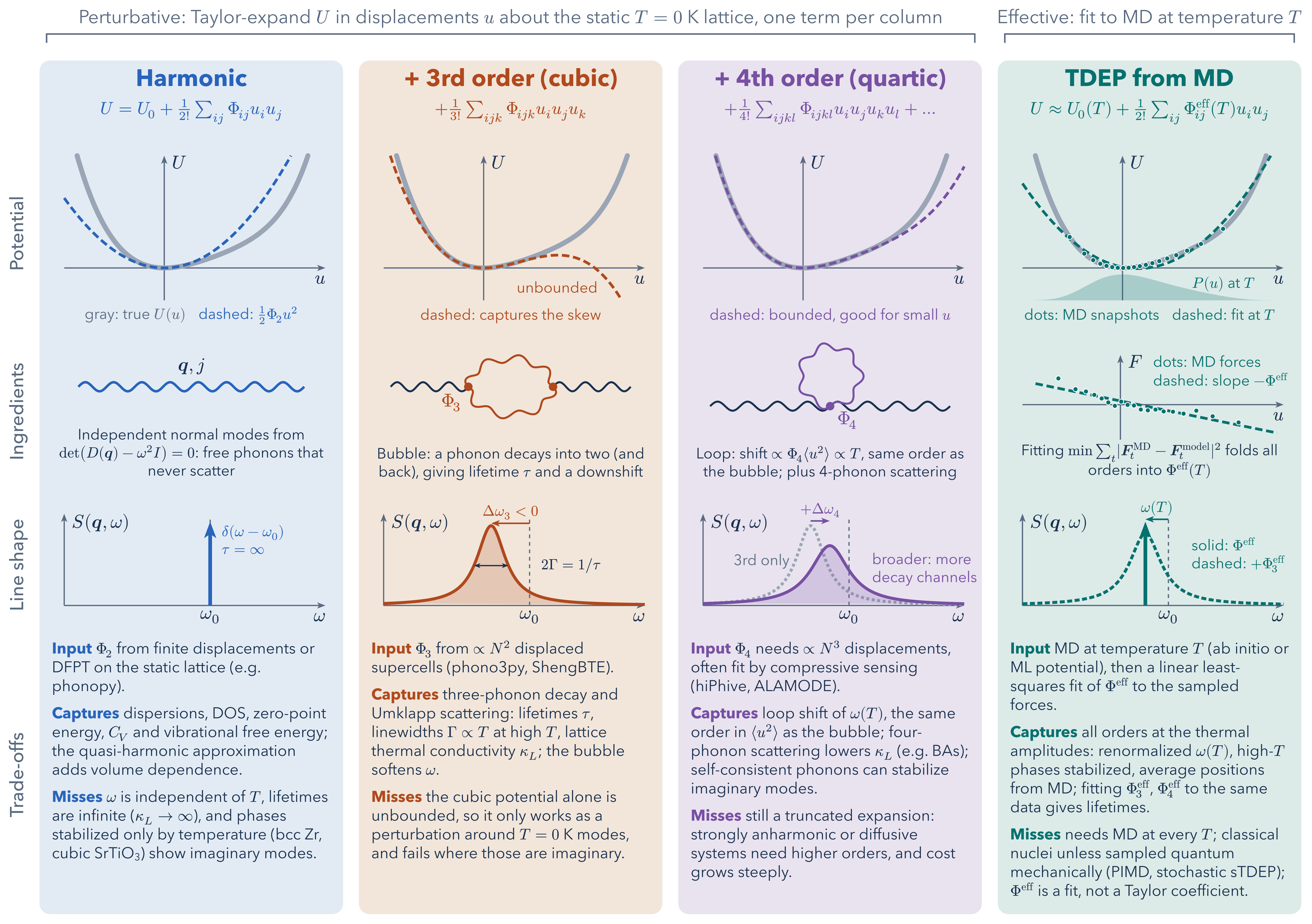
Four ways to model lattice vibrations, compared column by column. The first three Taylor-expand the potential energy in atomic displacements about the static K lattice, each adding one term: harmonic second-order force constants give independent normal modes with temperature-independent frequencies and infinite lifetimes, a delta-function line shape. Adding the cubic term lets a phonon decay into two (the bubble self-energy), which broadens the line to a width , softens the frequency and yields a finite lattice thermal conductivity, but the cubic potential alone is unbounded. The quartic term adds the loop self-energy, of the same order in as the bubble, which shifts the frequency with temperature, plus four-phonon scattering.
The temperature-dependent effective potential (TDEP) method instead runs molecular dynamics at temperature and least-squares fits effective force constants to the sampled forces. The best-fit parabola folds all anharmonic orders, at the amplitudes actually reached at that temperature, into renormalized frequencies, and can stabilize phases that are dynamically unstable in the harmonic approximation; effective third- and fourth-order constants fit to the same data give lifetimes. The potentials use a 1D toy on-site potential whose TDEP fit is computed from Boltzmann-sampled snapshots; the line shapes are schematic.
Download
Code
#import "@preview/cetz:0.5.3": canvas, draw
#import draw: circle, clip, content, line, rect

// Harmonic, cubic and quartic Taylor terms vs TDEP force constants fit to MD forces. Potentials
// use a 1D toy U(u) (u^6 stands in for higher orders); the TDEP column least-squares fits forces
// at Boltzmann-sampled u (k_B T = 0.5). Line shapes are schematic.
// https://doi.org/10.1103/PhysRevB.84.180301 https://doi.org/10.1103/PhysRevB.93.045202
#set page(width: auto, height: auto, margin: 8pt, fill: none)
#let (ink, muted, truth) = (rgb("#19304E"), rgb("#5A6A80"), rgb("#9AA6B5"))
#set text(font: "Avenir Next", size: 15pt, fill: ink)
#set par(leading: 0.5em)
#let colors = ("#2864BB", "#B04A1C", "#7750A3", "#06716E").map(rgb)
#let fills = ("#E2EAF4", "#F2E6DB", "#E9E3F0", "#DCEBE7").map(rgb)

// U(u) = sum c_k u^(k+2); its first 1, 2, 3 terms are the harmonic, cubic and quartic fits
#let cs = (0.5, -0.25, 0.06, 0, 0.003)
#let poly(n) = u => cs.slice(0, n).rev().fold(0, (acc, c) => acc * u + c) * u * u
#let U = poly(5)
#let force(u) = -cs.enumerate().rev().fold(0, (acc, (k, c)) => acc * u + (k + 2) * c) * u
// "MD snapshots": Boltzmann quantiles plus deterministic noise standing in for other atoms
#let (kT, n-md, grid) = (0.5, 19, range(3001).map(idx => -3 + 7.5 * idx / 3000))
#let cdf = grid.fold((), (acc, u) => acc + (acc.at(-1, default: 0) + calc.exp(-U(u) / kT),))
#let md-u = range(n-md).map(idx => grid.at(cdf.position(c => c >= (idx + 0.5) / n-md * cdf.last())))
#let noise(idx) = 2 * calc.rem-euclid(calc.sin(idx * 12.9898 + 4.1) * 43758.5453, 1) - 1
#let md-F = md-u.enumerate().map(((idx, u)) => force(u) + 0.22 * noise(idx))
// TDEP fit F = -k (u - u_c); U0 matches the mean sampled energy. By equipartition
// k = k_B T / <du^2>, so anharmonicity softens and shifts the fit.
#let mean(xs) = xs.sum() / xs.len()
#let cov(xs, ys) = mean(xs.zip(ys).map(((x, y)) => (x - mean(xs)) * (y - mean(ys))))
#let k-eff = -cov(md-u, md-F) / cov(md-u, md-u)
#let u-c = mean(md-u) + mean(md-F) / k-eff
#let U0 = mean(md-u.map(u => U(u) - k-eff / 2 * calc.pow(u - u-c, 2)))
#let fits = (poly(1), poly(2), poly(3), u => U0 + k-eff / 2 * calc.pow(u - u-c, 2))
#assert(0.8 < k-eff and k-eff < 1 and 0.1 < u-c and u-c < 0.5, message: repr((k-eff, u-c)))

// Map data (x, y) in x-lim × y-lim onto a w × h box with lower-left corner o
#let mapper(o, w, h, (x0, x1), (y0, y1)) = ((x, y)) => (
  o.at(0) + (x - x0) / (x1 - x0) * w,
  o.at(1) + (y - y0) / (y1 - y0) * h,
)
#let tip(color, scale) = (end: "stealth", fill: color, scale: scale)
#let axes(P, (x0, x1), (y0, y1), x-label, y-label, y-axis-x: 0) = {
  line(P((x0, 0)), P((x1, 0)), stroke: muted + 1pt, mark: tip(muted, 0.7))
  line(P((y-axis-x, y0)), P((y-axis-x, y1)), stroke: muted + 1pt, mark: tip(muted, 0.7))
  content(P((x1, 0)), x-label, anchor: "north-east", padding: (top: 6pt))
  content(P((y-axis-x, y1)), y-label, anchor: "north-west", padding: (left: 6pt))
}
#let samples((x0, x1), n: 200) = range(n + 1).map(idx => x0 + (x1 - x0) * idx / n)
#let small(body, ..args) = text(size: 12pt, ..args, body)
#let label(P, at, c, body, anchor: "west") = content(P(at), small(fill: c, body), anchor: anchor)
#let dashed(color) = (paint: color, thickness: 2.2pt, dash: (6pt, 3pt))
#let marker(pos, color) = circle(pos, radius: 0.07, fill: color, stroke: white + 0.6pt)

// Phonon propagator: a sine wave along the parametric curve p(t), t in [0, 1]
#let wavy(p, waves: 5, amp: 0.13, color: ink, width: 1.6pt) = line(
  ..range(waves * 16 + 1).map(idx => {
    let t = idx / (waves * 16)
    let ((x1, y1), (x2, y2)) = (p(calc.max(t - 1e-3, 0)), p(calc.min(t + 1e-3, 1)))
    let shift = amp * calc.sin(2 * calc.pi * waves * t) / calc.norm(x2 - x1, y2 - y1)
    let (x, y) = p(t)
    (x - (y2 - y1) * shift, y + (x2 - x1) * shift)
  }),
  stroke: color + width,
)
#let straight(a, b) = t => a.zip(b).map(((s, e)) => s + (e - s) * t)
#let arc((x, y), rx, ry, a, d) = t => (x + rx * calc.cos(a + d * t), y + ry * calc.sin(a + d * t))

// Spectral function S(q, omega): Lorentzian of half width g (g = 0.045 peaks at 1) or delta spike
#let lorentz(P, x0, g, color, dash: none) = line(
  ..samples((0.62, 1.3)).map(x => P((x, 0.045 * g / (calc.pow(x - x0, 2) + g * g)))),
  stroke: (paint: color, thickness: 2.4pt, dash: dash),
  fill: if dash == none { color.transparentize(80%) },
)
#let spike(P, x, color) = line(P((x, 0)), P((x, 1.05)), stroke: color + 3pt, mark: tip(color, 0.9))
#let shift(P, from, to, height, color, body) = {
  line(P((from, height)), P((to, height)), stroke: color + 1.3pt, mark: tip(color, 0.6))
  content(P(((from + to) / 2, height)), small(body, fill: color), anchor: "south", padding: 3pt)
}

// Layout: four 8.6 cm columns; rows of potentials, ingredients, line shapes and trade-offs
#let col-x(idx) = 1.1 + idx * 9.05
#let col-mid(idx) = col-x(idx) + 4.3
#let (u-lim, v-lim) = ((-1.8, 2.9), (-0.75, 2.6))
#let P-pot(idx) = mapper((col-x(idx) + 0.7, -8.35), 7.4, 4.1, u-lim, v-lim)
#let P-spec(idx) = mapper((col-x(idx) + 0.7, -17), 7.4, 2.6, (0.62, 1.3), (0, 1.15))

#canvas(length: 1cm, {
  // Scope headers: perturbative Taylor expansion vs effective fit
  let headers = (
    [Perturbative: Taylor-expand $U$ in displacements $u$ about the static $T = 0$ K lattice, one term per column],
    [Effective: fit to MD at temperature $T$],
  )
  for ((c0, c1), body) in ((0, 2), (3, 3)).zip(headers) {
    let (x0, x1) = (col-x(c0) + 0.2, col-x(c1) + 8.4)
    line((x0, -1.05), (x0, -0.8), (x1, -0.8), (x1, -1.05), stroke: muted + 1.2pt)
    content(((x0 + x1) / 2, -0.62), text(fill: muted, body), anchor: "south")
  }
  let titles = ([Harmonic], [\+ 3rd order (cubic)], [\+ 4th order (quartic)], [TDEP from MD])
  let terms = (
    $U = U_0 + 1 / 2! sum_(i j) Phi_(i j) u_i u_j$,
    $+ 1 / 3! sum_(i j k) Phi_(i j k) u_i u_j u_k$,
    $+ 1 / 4! sum_(i j k l) Phi_(i j k l) u_i u_j u_k u_l + dots$,
    $U approx U_0(T) + 1 / 2! sum_(i j) Phi_(i j)^"eff" (T) u_i u_j$,
  )
  let pot-captions = (
    [#text(fill: muted)[gray: true $U(u)$] #h(0.6em) dashed: $1/2 Phi_2 u^2$],
    [dashed: captures the skew],
    [dashed: bounded, good for small $u$],
    [dots: MD snapshots #h(0.6em) dashed: fit at $T$],
  )
  let row-labels = ([Potential], [Ingredients], [Line shape], [Trade-offs])
  for (y, body) in (-6.45, -11.5, -15.85, -21.8).zip(row-labels) {
    content((0.45, y), rotate(-90deg, reflow: true, text(fill: muted, weight: "medium", body)))
  }
  for (idx, color) in colors.enumerate() {
    let (x0, title) = (col-x(idx), text(19pt, weight: "bold", fill: color, titles.at(idx)))
    rect((x0, -1.55), (x0 + 8.6, -25.75), fill: fills.at(idx), stroke: none, radius: 0.3)
    content((col-mid(idx), -1.8), title, anchor: "north")
    content((col-mid(idx), -3), text(size: 14pt, fill: color, terms.at(idx)))
    // Row 1: true potential (gray) vs the model (dashed)
    let P = P-pot(idx)
    let curve(f) = samples(u-lim).map(u => P((u, f(u))))
    axes(P, u-lim, v-lim, $u$, $U$)
    clip(rect(P((u-lim.at(0), v-lim.at(0))), P((u-lim.at(1), v-lim.at(1)))), {
      line(..curve(U), stroke: (paint: truth, thickness: 4pt, cap: "round"))
      line(..curve(fits.at(idx)), stroke: dashed(color))
    })
    content((col-mid(idx), -8.8), small(fill: color, pot-captions.at(idx)))
    // Row 3: spectral function axes with the harmonic frequency omega_0
    let P = P-spec(idx)
    axes(P, (0.62, 1.3), (0, 1.15), $omega$, $S(bold(q), omega)$, y-axis-x: 0.62)
    line(P((1, 0)), P((1, 1.08)), stroke: (paint: muted, thickness: 1pt, dash: "dashed"))
    content(P((1, 0)), $omega_0$, anchor: "north", padding: (top: 4pt))
    // Row 4: inputs, captured physics and limitations
    let hd(body) = text(fill: color, strong(body))
    let notes = (
      [#hd[Input] $Phi_2$ from finite displacements or DFPT on the static lattice (e.g. phonopy). #v(-2pt) #hd[Captures] dispersions, DOS, zero-point energy, $C_V$ and vibrational free energy; the quasi-harmonic approximation adds volume dependence. #v(-2pt) #hd[Misses] $omega$ is independent of $T$, lifetimes are infinite ($kappa_L -> oo$), and phases stabilized only by temperature (bcc Zr, cubic SrTiO#sub[3]) show imaginary modes.],
      [#hd[Input] $Phi_3$ from $prop N^2$ displaced supercells (phono3py, ShengBTE). #v(-2pt) #hd[Captures] three-phonon decay and Umklapp scattering: lifetimes $tau$, linewidths $Gamma prop T$ at high $T$, lattice thermal conductivity $kappa_L$; the bubble softens $omega$. #v(-2pt) #hd[Misses] the cubic potential alone is unbounded, so it only works as a perturbation around $T = 0$ K modes, and fails where those are imaginary.],
      [#hd[Input] $Phi_4$ needs $prop N^3$ displacements, often fit by compressive sensing (hiPhive, ALAMODE). #v(-2pt) #hd[Captures] loop shift of $omega(T)$, the same order in $chevron.l u^2 chevron.r$ as the bubble; four-phonon scattering lowers $kappa_L$ (e.g. BAs); self-consistent phonons can stabilize imaginary modes. #v(-2pt) #hd[Misses] still a truncated expansion: strongly anharmonic or diffusive systems need higher orders, and cost grows steeply.],
      [#hd[Input] MD at temperature $T$ (ab initio or ML potential), then a linear least-squares fit of $Phi^"eff"$ to the sampled forces. #v(-2pt) #hd[Captures] all orders at the thermal amplitudes: renormalized $omega(T)$, high-$T$ phases stabilized, average positions from MD; fitting $Phi_3^"eff"$, $Phi_4^"eff"$ to the same data gives lifetimes. #v(-2pt) #hd[Misses] needs MD at every $T$; classical nuclei unless sampled quantum mechanically (PIMD, stochastic sTDEP); $Phi^"eff"$ is a fit, not a Taylor coefficient.],
    )
    let notes-box = box(width: 7.9cm, height: 7.2cm, text(size: 12.5pt, notes.at(idx)))
    content((col-x(idx) + 0.35, -18.05), notes-box, anchor: "north-west")
  }

  // Row 1 extras: the unbounded cubic and TDEP's thermal sampling P(u)
  label(P-pot(1), (2.05, -0.45), colors.at(1), [unbounded], anchor: "east")
  let (P, color) = (P-pot(3), colors.at(3))
  let strip = samples(u-lim, n: 120).map(u => P((u, -0.75 + 0.6 * calc.exp(-U(u) / kT))))
  line(..strip, fill: color.transparentize(75%), stroke: none)
  label(P, (1.25, -0.38), color)[$P(u)$ at $T$]
  for u in md-u { marker(P((u, U(u))), color) }

  // Row 2: what each model contains
  let (cx, y) = (col-mid(0), -10.8)
  let vertex(pos, color) = circle(pos, radius: 0.12, fill: color, stroke: none)
  wavy(straight((cx - 3.2, y), (cx + 3.2, y)), waves: 8, color: colors.at(0), width: 2pt)
  content((cx, y + 0.35), $bold(q), j$, anchor: "south")
  let (cx, color) = (col-mid(1), colors.at(1))
  wavy(straight((cx - 3.4, y), (cx - 1.2, y)), waves: 3)
  wavy(straight((cx + 1.2, y), (cx + 3.4, y)), waves: 3)
  for ry in (0.8, -0.8) {
    wavy(arc((cx, y), 1.2, ry, 180deg, -180deg), waves: 4, amp: 0.11, color: color)
  }
  for x in (cx - 1.2, cx + 1.2) { vertex((x, y), color) }
  content((cx - 1.4, y - 0.2), text(fill: color)[$Phi_3$], anchor: "north-east")
  let (cx, color, vy, r) = (col-mid(2), colors.at(2), y - 0.55, 0.85)
  wavy(straight((cx - 3.4, vy), (cx, vy)), waves: 4)
  wavy(straight((cx, vy), (cx + 3.4, vy)), waves: 4)
  wavy(arc((cx, vy + r), r, r, -90deg, 360deg), waves: 7, amp: 0.1, color: color)
  vertex((cx, vy), color)
  content((cx + 0.2, vy - 0.15), text(fill: color)[$Phi_4$], anchor: "north-west")
  // TDEP: force vs displacement of the MD snapshots and the least-squares line
  let (color, f-lim) = (colors.at(3), (-2.4, 3.4))
  let P = mapper((col-x(3) + 0.7, -12.3), 7.4, 2.4, (-1.5, 2.5), f-lim)
  axes(P, (-1.5, 2.5), f-lim, $u$, $F$)
  line(..(-1.3, 2.4).map(u => P((u, -k-eff * (u - u-c)))), stroke: dashed(color))
  for (u, F) in md-u.zip(md-F) { marker(P((u, F)), color) }
  label(P, (0.5, 1.55), color)[dashed: slope $-Phi^"eff"$]
  label(P, (0.5, 2.95), color)[dots: MD forces]
  let captions = (
    [Independent normal modes from $det(D(bold(q)) - omega^2 I) = 0$: free phonons that never scatter],
    [Bubble: a phonon decays into two (and back), giving lifetime $tau$ and a downshift],
    [Loop: shift $prop Phi_4 chevron.l u^2 chevron.r prop T$, same order as the bubble; plus 4-phonon scattering],
    [Fitting $min sum_t |bold(F)_t^"MD" - bold(F)_t^"model"|^2$ folds all orders into $Phi^"eff" (T)$],
  )
  for (idx, body) in captions.enumerate() {
    content((col-mid(idx), -13.55), box(width: 8cm, align(center, small(body))), anchor: "south")
  }

  // Row 3: line shapes of one mode q
  let (P, color) = (P-spec(0), colors.at(0))
  spike(P, 1, color)
  label(P, (1.03, 0.8), color)[$delta(omega - omega_0)$\ $tau = oo$]
  let (P, color) = (P-spec(1), colors.at(1))
  lorentz(P, 0.9, 0.045, color)
  let both-tips = (start: "stealth", end: "stealth", fill: ink, scale: 0.45)
  line(P((0.855, 0.5)), P((0.945, 0.5)), stroke: ink + 1pt, mark: both-tips)
  label(P, (1.03, 0.5), ink)[$2 Gamma = 1 slash tau$]
  shift(P, 1, 0.9, 1.03, color, $Delta omega_3 < 0$)
  let (P, color) = (P-spec(2), colors.at(2))
  lorentz(P, 0.9, 0.045, truth, dash: "dotted")
  label(P, (0.845, 0.55), muted, [3rd only], anchor: "east")
  lorentz(P, 0.95, 0.06, color)
  shift(P, 0.9, 0.95, 1.06, color, $+ Delta omega_4$)
  label(P, (1.06, 0.45), color)[broader: more\ decay channels]
  let (P, color) = (P-spec(3), colors.at(3))
  lorentz(P, 0.94, 0.05, color, dash: (4pt, 2pt))
  spike(P, 0.94, color)
  shift(P, 1, 0.94, 1.08, color, $omega(T)$)
  label(P, (1.06, 0.62), color)[solid: $Phi^"eff"$\ dashed: $+ Phi_3^"eff"$]
})