Normalizing Flows
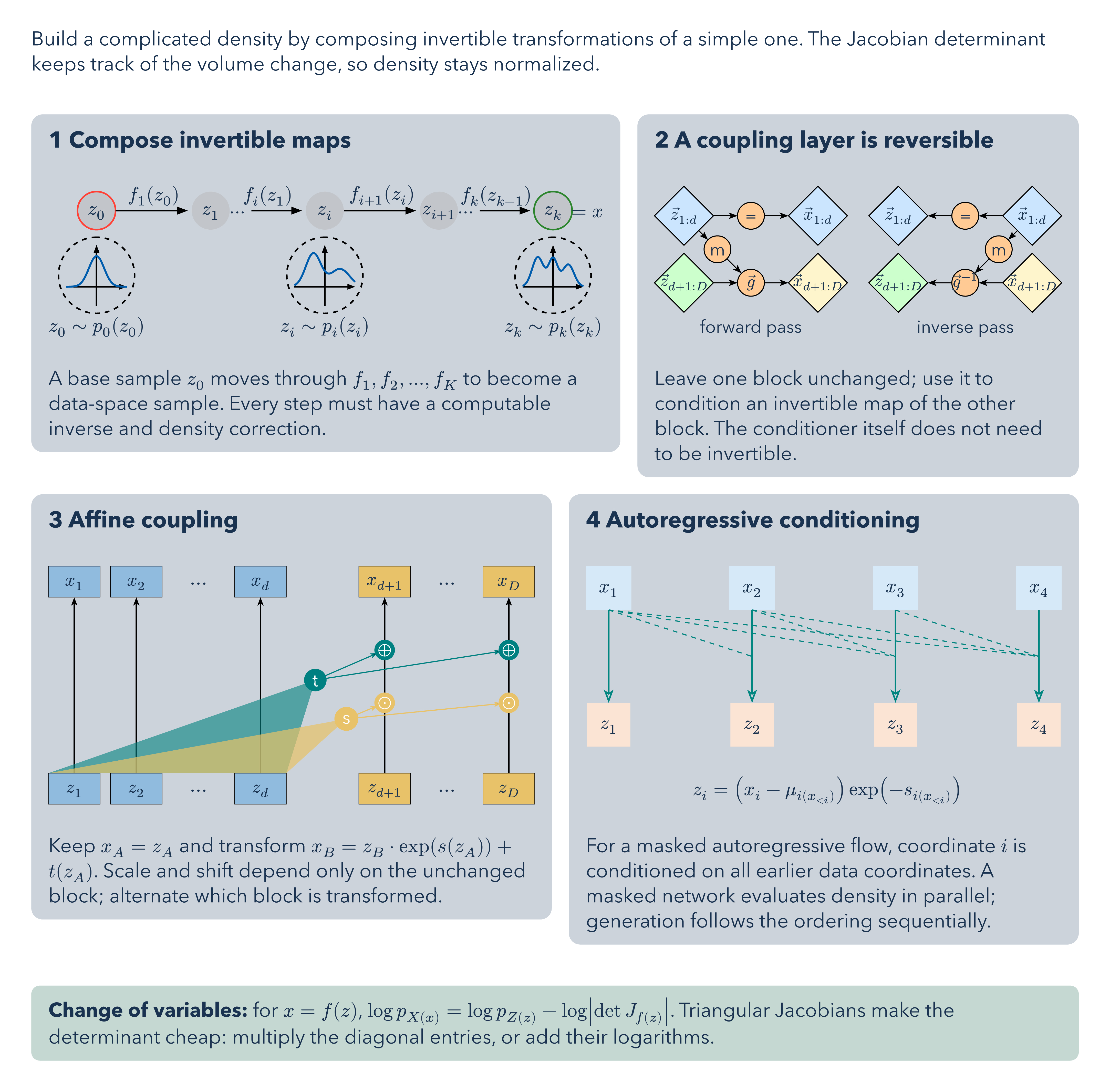
Build a complicated density by composing invertible transformations of a simple one. The Jacobian determinant keeps track of the volume change, so density stays normalized.
Sources: Real NVP and Masked Autoregressive Flow.
Download
Code
normalizing-flows.typ (377 lines)
#import "@preview/cetz:0.5.2": canvas, draw
#import "@preview/cetz-plot:0.1.4": plot
#import draw: circle, content, group, hobby, line, polygon, rect, translate
#let label-size = 12pt
#let paragraph-size = 14pt
#let heading-size = 16pt

#let card_body(title, body, caption) = block(
  width: 100%,
  inset: 12pt,
  radius: 8pt,
  fill: rgb("#cdd3da"),
  breakable: false,
)[
  #text(size: heading-size, weight: "bold", title)
  #v(8pt)
  // Measure unconstrained artwork before scaling, including content wider than its card.
  #layout(size => {
    let artwork = text(size: label-size, body)
    std.scale(size.width / measure(artwork).width * 100%, reflow: true, artwork)
  })
  #v(7pt)
  #text(size: paragraph-size, caption)
]

#let card-grid(columns: 2, ..cards) = layout(size => {
  let rows = cards
    .pos()
    .chunks(columns)
    .map(row => {
      let ratios = row.map(card => {
        let bounds = measure(text(size: label-size, card.at(1)))
        bounds.width / bounds.height
      })
      let available = size.width - 12pt * (row.len() - 1) - 24pt * row.len()
      grid(
        columns: ratios.map(ratio => 24pt + available * ratio / ratios.sum()),
        gutter: 12pt,
        ..row.map(args => card_body(..args)),
      )
    })
  stack(dir: ttb, spacing: 12pt, ..rows)
})

#let takeaway(body) = block(
  width: 100%,
  inset: 12pt,
  radius: 6pt,
  fill: rgb("#c6d8d2"),
  breakable: false,
  text(size: paragraph-size, body),
)

#set page(width: 780pt, height: auto, margin: 22pt, fill: none)
#set text(font: "Avenir Next", size: paragraph-size, fill: rgb("#19324f"))
#set par(leading: 0.55em)

// === 1  Compose invertible maps ===
#let figure-0 = [
  // Helper functions for probability distributions
  #let gaussian(x, mu: 0, sigma: 0.2) = (
    (1 / (sigma * calc.sqrt(2 * calc.pi))) * calc.exp(-0.5 * calc.pow((x - mu) / sigma, 2))
  )

  #let mixture(x, params) = {
    let sum = 0
    for (weight, mu, sigma) in params {
      sum += weight * gaussian(x, mu: mu, sigma: sigma)
    }
    return sum
  }

  // Distribution functions
  #let p0(x) = 0.55 * gaussian(x, mu: 0, sigma: 0.2)
  #let pi(x) = mixture(x, ((0.6, -0.3, 0.2), (0.4, 0.4, 0.25)))
  #let pk(x) = mixture(x, ((0.4, -0.4, 0.15), (0.3, 0, 0.12), (0.3, 0.4, 0.15)))

  #let draw-distro(x, y, dist-fn, name: none) = {
    circle((x, y + 0.3), radius: 1, stroke: (dash: "dashed"), name: name)

    line((x - 0.8, y), (x + 0.8, y), mark: (end: ">", scale: 0.5, fill: black))
    line((x, y - 0.5), (x, y + 1.1), mark: (end: ">", scale: 0.5, fill: black))

    let plot-size = (1.6, 1.1)

    group({
      translate((x - 0.8, y))
      plot.plot(size: plot-size, axis-style: none, y-min: 0, y-max: 1.5, {
        plot.add(
          style: (stroke: blue.darken(20%) + 1.2pt),
          domain: (-0.8, 0.8),
          samples: 100,
          dist-fn,
        )
      })
    })
  }

  #canvas(length: .82cm, {
    // Constants for layout
    let node-spacing = 3
    let y-base = 0
    let y-distro = y-base - 2 // vertical offset for distributions

    // Helper function for z-nodes
    let z-node(x, label, special: none, name: none) = {
      circle(
        fill: gray.transparentize(70%),
        (x, y-base),
        radius: 0.5,
        stroke: special,
        name: name,
      )
      content(name, label)
    }

    // Draw all nodes first
    z-node(0, $z_0$, special: red, name: "z0")
    z-node(node-spacing, $z_1$, name: "z1")
    z-node(2 * node-spacing, $z_i$, name: "zi")
    z-node(3 * node-spacing, $z_(i+1)$, name: "zi1")
    z-node(4 * node-spacing, $z_k$, special: rgb("#2d862d"), name: "zk")

    // Then add dots
    content((rel: (0.7, 0), to: "z1"), $dots.c$, name: "dots1", padding: 4pt)
    content((rel: (0.7, 0), to: "zi1"), $dots.c$, name: "dots2", padding: 4pt)
    content((rel: (0.9, 0), to: "zk"), $= x$)

    let arrow-style = (end: ">", fill: black, scale: 0.8, offset: 0.1)
    for (from, to, edge, position, label, label-name) in (
      ("z0", "z1", "z0-z1", "mid", $f_(1)(z_0)$, "f1"),
      ("dots1.east", "zi", "z1-zi", "30%", $f_i (z_1)$, "fi"),
      ("zi", "zi1", "zi-zi1", "mid", $f_(i+1) (z_i)$, "fi1"),
      ("dots2.east", "zk", "zi1-zk", "30%", $f_k (z_(k-1))$, "fk"),
    ) {
      line(from, to, mark: arrow-style, name: edge)
      content(edge + "." + position, label, name: label-name, anchor: "south", padding: (
        bottom: 3pt,
      ))
    }

    draw-distro(0, y-distro, p0, name: "d0")
    content("d0.south", $z_0 ~ p_(0)(z_0)$, anchor: "north", padding: (top: 3pt))

    draw-distro(2 * node-spacing, y-distro, pi, name: "di")
    content("di.south", $z_i ~ p_(i)(z_i)$, anchor: "north", padding: (top: 3pt))

    draw-distro(4 * node-spacing, y-distro, pk, name: "dk")
    content("dk.south", $z_k ~ p_(k)(z_k)$, anchor: "north", padding: (top: 3pt))
  })
]

// === 2  A coupling layer is reversible ===
#let figure-1 = canvas(length: .65cm, {
  let spacing = (node: 2.5, row: 2.5)

  // Node styles
  let arrow-style = (
    mark: (end: "stealth", fill: black, scale: 0.75),
    stroke: 0.7pt,
  )

  let diamond(pos, name, label, fill: none) = {
    polygon(pos, 4, radius: 1.1, angle: 90deg, stroke: 0.7pt, fill: fill, name: name)
    content(pos, label, anchor: "center")
  }

  let circle-node(pos, name, label) = {
    circle(
      pos,
      radius: 0.5,
      name: name,
      stroke: 0.7pt,
      fill: rgb("#ffa64d").lighten(40%),
    )
    content(pos, label, anchor: "center")
  }

  // The inverse uses the same two rows, with reversed data arrows and conditioning from x.
  for (prefix, offset, inverse) in (
    ("forward-", 0, false),
    ("inverse-", 3.2 * spacing.node, true),
  ) {
    let name(node) = prefix + node
    let at(column, row) = (offset + column * spacing.node, -row * spacing.row)
    diamond(at(0, 0), name("z1"), $arrow(z)_(1:d)$, fill: rgb("#cce5ff"))
    circle-node(at(1, 0), name("eq"), "=")
    diamond(at(2, 0), name("x1"), $arrow(x)_(1:d)$, fill: rgb("#cce5ff"))
    diamond(at(0, 1), name("z2"), $arrow(z)_(d+1:D)$, fill: rgb("#ccffcc"))
    circle-node(at(1, 1), name("g"), if inverse { $arrow(g)^(-1)$ } else { $arrow(g)$ })
    diamond(at(2, 1), name("x2"), $arrow(x)_(d+1:D)$, fill: rgb("#fff5cc"))
    circle-node(at(if inverse { 1.5 } else { 0.5 }, 0.5), name("m"), "m")

    for (left, right) in (("z1", "eq"), ("eq", "x1"), ("z2", "g"), ("g", "x2")) {
      let (from, to) = if inverse { (right, left) } else { (left, right) }
      line(name(from), name(to), ..arrow-style)
    }
    line(name(if inverse { "x1" } else { "z1" }), name("m"), ..arrow-style)
    line(name("m"), name("g"), ..arrow-style)
    content(
      (rel: (0, -1.4), to: name("g")),
      if inverse { [inverse pass] } else { [forward pass] },
      anchor: "north",
    )
  }
})

// === 3  Affine coupling ===
#let figure-2 = canvas(length: 1.2cm, {
  let node-width = 1
  let node-height = 0.6
  let horiz-sep = 1.2
  let vert-sep = 4
  let arrow-style = (end: "stealth", fill: black, scale: .5)
  let (orange, blue, teal) = (rgb("#e8c268"), rgb("#63a7e390"), rgb("#008080"))

  // Helper function for boxes
  let box(pos, body, fill: none, name: none) = {
    rect(
      pos,
      (rel: (node-width, node-height)),
      fill: fill,
      stroke: 0.3pt,
      name: name,
    )
    content(name, body)
  }

  for (prefix, y-pos, labels) in (
    ("x", 0, ($x_1$, $x_2$, $x_d$, $x_(d+1)$, $x_D$)),
    ("z", -vert-sep, ($z_1$, $z_2$, $z_d$, $z_(d+1)$, $z_D$)),
  ) {
    let nodes = (
      (0, prefix + "1", labels.at(0), blue),
      (horiz-sep, prefix + "2", labels.at(1), blue),
      (3 * horiz-sep, prefix + "d", labels.at(2), blue),
      (5 * horiz-sep, prefix + "d-plus-1", labels.at(3), orange),
      (7 * horiz-sep, prefix + "D", labels.at(4), orange),
    )
    for (x-pos, name, label, fill) in nodes {
      box((x-pos, y-pos), label, fill: fill, name: name)
    }
    content((prefix + "2", 50%, prefix + "d"), text(size: 14pt)[$dots.c$], name: prefix + "dots1")
    content(
      (prefix + "d-plus-1", 50%, prefix + "D"),
      text(size: 14pt)[$dots.c$],
      name: prefix + "dots2",
    )
  }

  // Vertical connecting lines
  for (suffix, line-name) in (
    ("1", "line1"),
    ("2", "line2"),
    ("d", "lined"),
    ("d-plus-1", "line-d-plus-1"),
    ("D", "lineD"),
  ) { line("z" + suffix, "x" + suffix, mark: arrow-style, name: line-name) }

  // Scale and translate functions: a labeled circle and its conditioning triangle.
  for (name, pos, baseline, color, transparency) in (
    ("t", (4.3 * horiz-sep, 0.4 * -vert-sep), 0pt, teal, 40%),
    ("s", (rel: (.6, -.75), to: "t-circle"), -1pt, orange, 30%),
  ) {
    content(
      pos,
      text(fill: white, baseline: baseline, name),
      frame: "circle",
      name: name + "-circle",
      stroke: none,
      fill: color,
      padding: 2pt,
    )
    line(
      "z1.north-west",
      name + "-circle",
      "zd.north-east",
      fill: color.transparentize(transparency),
      close: true,
      stroke: none,
      name: name + "-triangle",
    )
  }

  // Operation circles
  for line-name in ("line-d-plus-1", "lineD") {
    for (op, (color, label, pos)) in (
      "odot": (orange, $dot.o$, "40%"),
      "oplus": (teal, $plus.o$, "70%"),
    ).pairs() {
      content(
        line-name + "." + pos,
        text(fill: white, baseline: -.2pt)[#label],
        frame: "circle",
        name: line-name + "-" + op,
        stroke: none,
        fill: color,
        padding: .1pt,
      )
    }
  }

  // Connect s and t to operations.
  for line-name in ("line-d-plus-1", "lineD") {
    for (source, operation, color) in (("s", "odot", orange), ("t", "oplus", teal)) {
      hobby(
        source + "-circle",
        line-name + "-" + operation,
        mark: (..arrow-style, offset: 5pt),
        stroke: color + 0.75pt,
      )
    }
  }
})

// === 4  Autoregressive conditioning ===
#let figure-3 = canvas(length: 1.5cm, {
  for idx in range(4) {
    for (prefix, row, label, fill) in (
      ("x", 0, $x_#(idx + 1)$, rgb("#d6e9f8")),
      ("z", -2, $z_#(idx + 1)$, rgb("#fbe4d4")),
    ) {
      draw.content(
        (idx * 2.1, row),
        label,
        name: prefix + str(idx),
        frame: "rect",
        padding: 8pt,
        fill: fill,
        stroke: none,
      )
    }
    draw.line(
      "x" + str(idx) + ".south",
      "z" + str(idx) + ".north",
      stroke: rgb("#008580") + 1pt,
      mark: (end: "stealth"),
    )
    for earlier in range(idx) {
      draw.line("x" + str(earlier) + ".south", (idx * 2.1, -1), stroke: (
        paint: rgb("#008580"),
        thickness: .7pt,
        dash: "dashed",
      ))
    }
  }
  draw.content((3.2, -3), $z_i=(x_i-mu_i(x_(<i))) exp(-s_i(x_(<i)))$)
})

Build a complicated density by composing invertible transformations of a simple one. The Jacobian determinant keeps track of the volume change, so density stays normalized.
#v(14pt)
#card-grid(
  (
    [1  Compose invertible maps],
    figure-0,
    [A base sample $z_0$ moves through $f_1, f_2, dots, f_K$ to become a data-space sample. Every step must have a computable inverse and density correction.],
  ),
  (
    [2  A coupling layer is reversible],
    figure-1,
    [Leave one block unchanged; use it to condition an invertible map of the other block. The conditioner itself does not need to be invertible.],
  ),

  (
    [3  Affine coupling],
    figure-2,
    [Keep $x_A=z_A$ and transform $x_B=z_B dot exp(s(z_A))+t(z_A)$. Scale and shift depend only on the unchanged block; alternate which block is transformed.],
  ),
  (
    [4  Autoregressive conditioning],
    figure-3,
    [For a masked autoregressive flow, coordinate $i$ is conditioned on all earlier data coordinates. A masked network evaluates density in parallel; generation follows the ordering sequentially.],
  ),
)
#v(12pt)
#takeaway[*Change of variables:* for $x=f(z)$, $log p_X(x)=log p_Z(z)-log abs(det J_f(z))$. Triangular Jacobians make the determinant cheap: multiply the diagonal entries, or add their logarithms.]