Particle Statistics
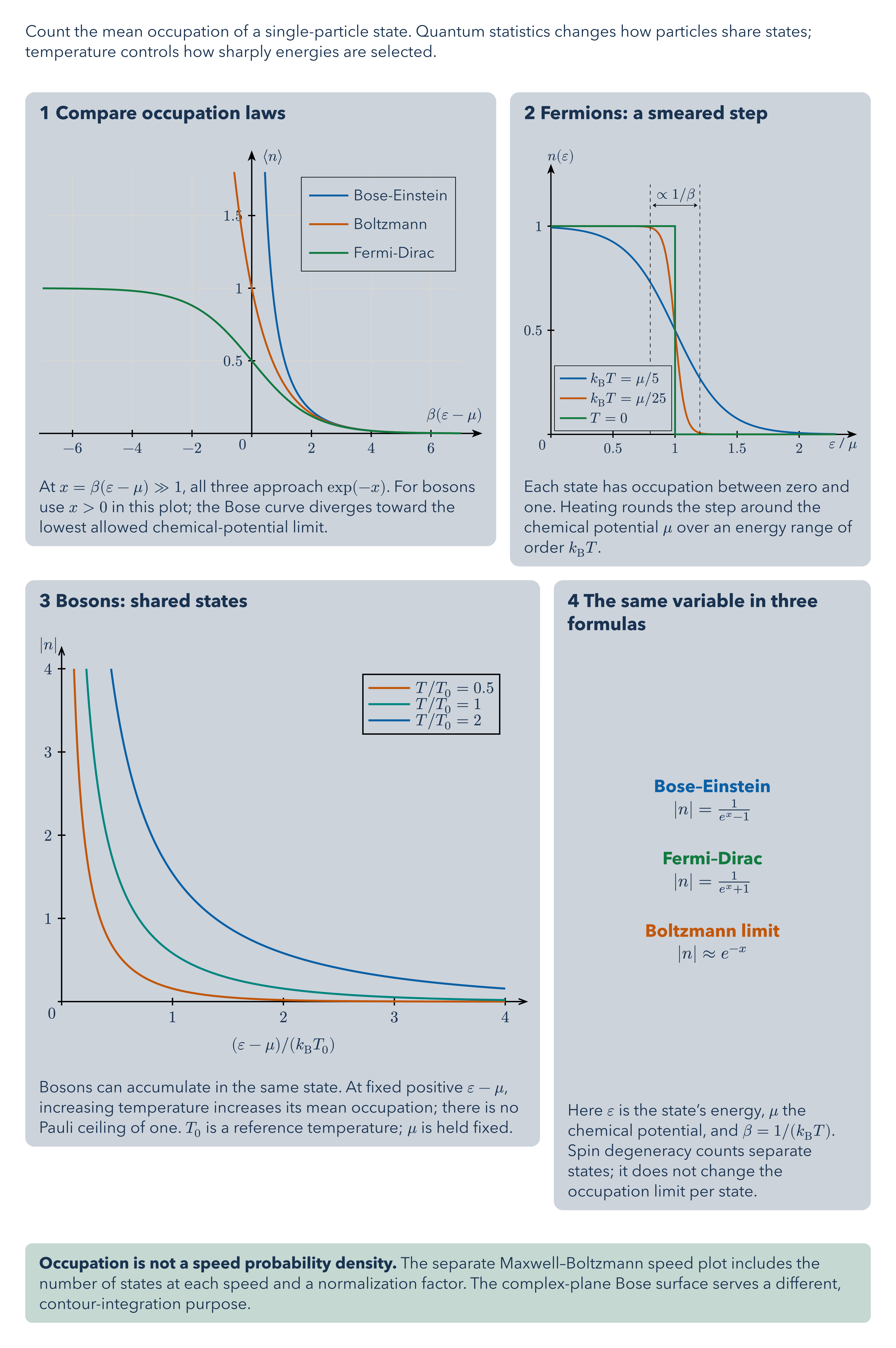
Count the mean occupation of a single-particle state. Quantum statistics changes how particles share states; temperature controls how sharply energies are selected.
Download
Code
particle-statistics.typ (246 lines)
#import "@preview/cetz:0.5.2": canvas, draw
#import "@preview/cetz-plot:0.1.4": plot
#import draw: content
#let label-size = 12pt
#let paragraph-size = 14pt
#let heading-size = 16pt

#let card_body(title, body, caption) = block(
  width: 100%,
  inset: 12pt,
  radius: 8pt,
  fill: rgb("#cdd3da"),
  breakable: false,
)[
  #text(size: heading-size, weight: "bold", title)
  #v(8pt)
  // Measure unconstrained artwork before scaling, including content wider than its card.
  #layout(size => {
    let artwork = text(size: label-size, body)
    std.scale(size.width / measure(artwork).width * 100%, reflow: true, artwork)
  })
  #v(7pt)
  #text(size: paragraph-size, caption)
]

#let card-grid(columns: 2, ..cards) = layout(size => {
  let rows = cards
    .pos()
    .chunks(columns)
    .map(row => {
      let ratios = row.map(card => {
        let bounds = measure(text(size: label-size, card.at(1)))
        bounds.width / bounds.height
      })
      let available = size.width - 12pt * (row.len() - 1) - 24pt * row.len()
      grid(
        columns: ratios.map(ratio => 24pt + available * ratio / ratios.sum()),
        gutter: 12pt,
        ..row.map(args => card_body(..args)),
      )
    })
  stack(dir: ttb, spacing: 12pt, ..rows)
})

#let takeaway(body) = block(
  width: 100%,
  inset: 12pt,
  radius: 6pt,
  fill: rgb("#c6d8d2"),
  breakable: false,
  text(size: paragraph-size, body),
)

#set page(width: 780pt, height: auto, margin: 22pt, fill: none)
#set text(font: "Avenir Next", size: paragraph-size, fill: rgb("#19324f"))
#set par(leading: 0.55em)

// Mean occupation per single-particle state; zero-point energy is not occupation.
#let bose-occupation(x) = {
  assert(x > 0, message: "Bose occupation requires epsilon > mu")
  1 / (calc.exp(x) - 1)
}
#let fermi-dirac(x) = 1 / (calc.exp(x) + 1)

// === 1  Compare occupation laws ===
#let figure-0 = [
  // Distribution functions
  #let boltzmann(x) = 1 / calc.exp(x)

  #canvas(length: 1.45cm, {
    draw.set-style(legend: (fill: rgb("#cdd3da")))
    let axis-mark = (end: "stealth", fill: black)
    draw.set-style(axes: (
      x: (mark: axis-mark, label: (anchor: "south-east", offset: -0.2)),
      y: (mark: axis-mark, label: (anchor: "north-west", offset: -0.2)),
    ))

    plot.plot(
      size: (8, 5),
      x-label: $beta (epsilon - mu)$,
      y-label: $chevron.l n chevron.r$,
      x-min: -7,
      x-max: 7,
      y-min: 0,
      y-max: 1.8,
      x-tick-step: 2,
      y-tick-step: 0.5,
      axis-style: "school-book",
      x-grid: true,
      y-grid: true,
      legend: "inner-north-east",
      // Compact legend with a thin border.
      legend-style: (item: (spacing: 0.15), padding: 0.15, stroke: 0.5pt),
      {
        // Start the Bose curve above zero, where its occupation diverges.
        for (label, distribution, color, minimum, samples) in (
          ("Bose-Einstein", bose-occupation, rgb("#0B5FA5"), 0.1, 200),
          ("Boltzmann", boltzmann, rgb("#C2570A"), -1, 100),
          ("Fermi-Dirac", fermi-dirac, rgb("#12793F"), -7, 100),
        ) {
          plot.add(
            style: (stroke: color + 1.5pt),
            domain: (minimum, 7),
            samples: samples,
            label: label,
            distribution,
          )
        }
      },
    )
  })
]

// === 2  Fermions: a smeared step ===
#let figure-1 = [
  #canvas(length: 1.04cm, {
    draw.set-style(legend: (fill: rgb("#cdd3da")))
    let axis-mark = (end: "stealth", fill: black)
    draw.set-style(axes: (
      x: (mark: axis-mark, label: (anchor: "north-east")),
      y: (mark: axis-mark, label: (anchor: "south-west")),
    ))

    plot.plot(
      size: (8, 7),
      x-label: [$epsilon$ / $mu$],
      y-label: $n(epsilon)$,
      x-min: 0,
      x-max: 2.3,
      y-min: 0,
      y-max: 1.2,
      x-tick-step: .5,
      y-tick-step: .5,
      y-ticks: (0.5, 1),
      axis-style: "left",
      legend: "inner-south-west",
      // Compact legend with a thin border.
      legend-style: (item: (spacing: 0.15), padding: 0.15, stroke: 0.5pt),
      {
        let chem-pot = 1

        for (beta, color) in ((5, rgb("#0B5FA5")), (25, rgb("#C2570A"))) {
          plot.add(
            style: (stroke: color + 1.5pt),
            domain: (0, 2.3),
            samples: 150,
            x => fermi-dirac(beta * (x - chem-pot)),
            label: $k_"B" T = mu \/ #beta$,
          )
        }

        // T = 0 (blue step function)
        let points = ((0, 1), (chem-pot, 1), (chem-pot, 0), (2.3, 0))
        plot.add(
          style: (stroke: rgb("#12793F") + 1.5pt),
          points,
          label: $T = 0$,
        )

        plot.add-vline(0.8, style: (stroke: (dash: "dashed", thickness: 0.5pt)))
        plot.add-vline(1.2, style: (stroke: (dash: "dashed", thickness: 0.5pt)))

        plot.add-hline(1.1, min: 0.8, max: 1.2, style: (
          stroke: (thickness: 0.5pt),
          mark: (symbol: "stealth", stroke: 0.5pt, fill: black, scale: .1),
        ))
      },
    )

    content((3.5, 6.5), $prop 1 \/ beta$, anchor: "south")
  })
]

// === 3  Bosons: shared states ===
#let figure-2 = canvas(length: 1.45cm, {
  draw.set-style(legend: (fill: rgb("#cdd3da")))
  plot.plot(
    size: (8, 6),
    x-min: 0,
    x-max: 4,
    y-min: 0,
    y-max: 4,
    x-label: none,
    y-label: $bar(n)$,
    x-tick-step: 1,
    y-tick-step: 1,
    axis-style: "left",
    legend: "inner-north-east",
    {
      for (temp, color) in ((0.5, rgb("#c2570a")), (1, rgb("#008580")), (2, rgb("#0b5fa5"))) {
        plot.add(
          style: (stroke: color + 1.5pt),
          domain: (0.03, 4),
          samples: 240,
          x => bose-occupation(x / temp),
          label: [$T \/ T_0 = #temp$],
        )
      }
    },
  )
  draw.content((4, -.8), $(epsilon-mu) \/ (k_"B" T_0)$)
})

// === 4  The same variable in three formulas ===
#let figure-3 = box(width: 230pt, height: 330pt)[
  #align(center + horizon)[
    #set text(size: paragraph-size)
    #text(fill: rgb("#0b5fa5"))[*Bose–Einstein*]\
    $bar(n) = 1/(e^x-1)$\
    #v(13pt)
    #text(fill: rgb("#12793f"))[*Fermi–Dirac*]\
    $bar(n) = 1/(e^x+1)$\
    #v(13pt)
    #text(fill: rgb("#c2570a"))[*Boltzmann limit*]\
    $bar(n) approx e^(-x)$
  ]
]

Count the mean occupation of a single-particle state. Quantum statistics changes how particles share states; temperature controls how sharply energies are selected.
#v(14pt)
#card-grid(
  (
    [1  Compare occupation laws],
    figure-0,
    [At $x=beta(epsilon-mu) >> 1$, all three approach $exp(-x)$. For bosons use $x>0$ in this plot; the Bose curve diverges toward the lowest allowed chemical-potential limit.],
  ),
  (
    [2  Fermions: a smeared step],
    figure-1,
    [Each state has occupation between zero and one. Heating rounds the step around the chemical potential $mu$ over an energy range of order $k_"B" T$.],
  ),

  (
    [3  Bosons: shared states],
    figure-2,
    [Bosons can accumulate in the same state. At fixed positive $epsilon-mu$, increasing temperature increases its mean occupation; there is no Pauli ceiling of one. $T_0$ is a reference temperature; $mu$ is held fixed.],
  ),
  (
    [4  The same variable in three formulas],
    figure-3,
    [Here $epsilon$ is the state’s energy, $mu$ the chemical potential, and $beta=1 \/ (k_"B" T)$. Spin degeneracy counts separate states; it does not change the occupation limit per state.],
  ),
)
#v(12pt)
#takeaway[*Occupation is not a speed probability density.* The separate Maxwell–Boltzmann speed plot includes the number of states at each speed and a normalization factor. The complex-plane Bose surface serves a different, contour-integration purpose.]