XC Functional
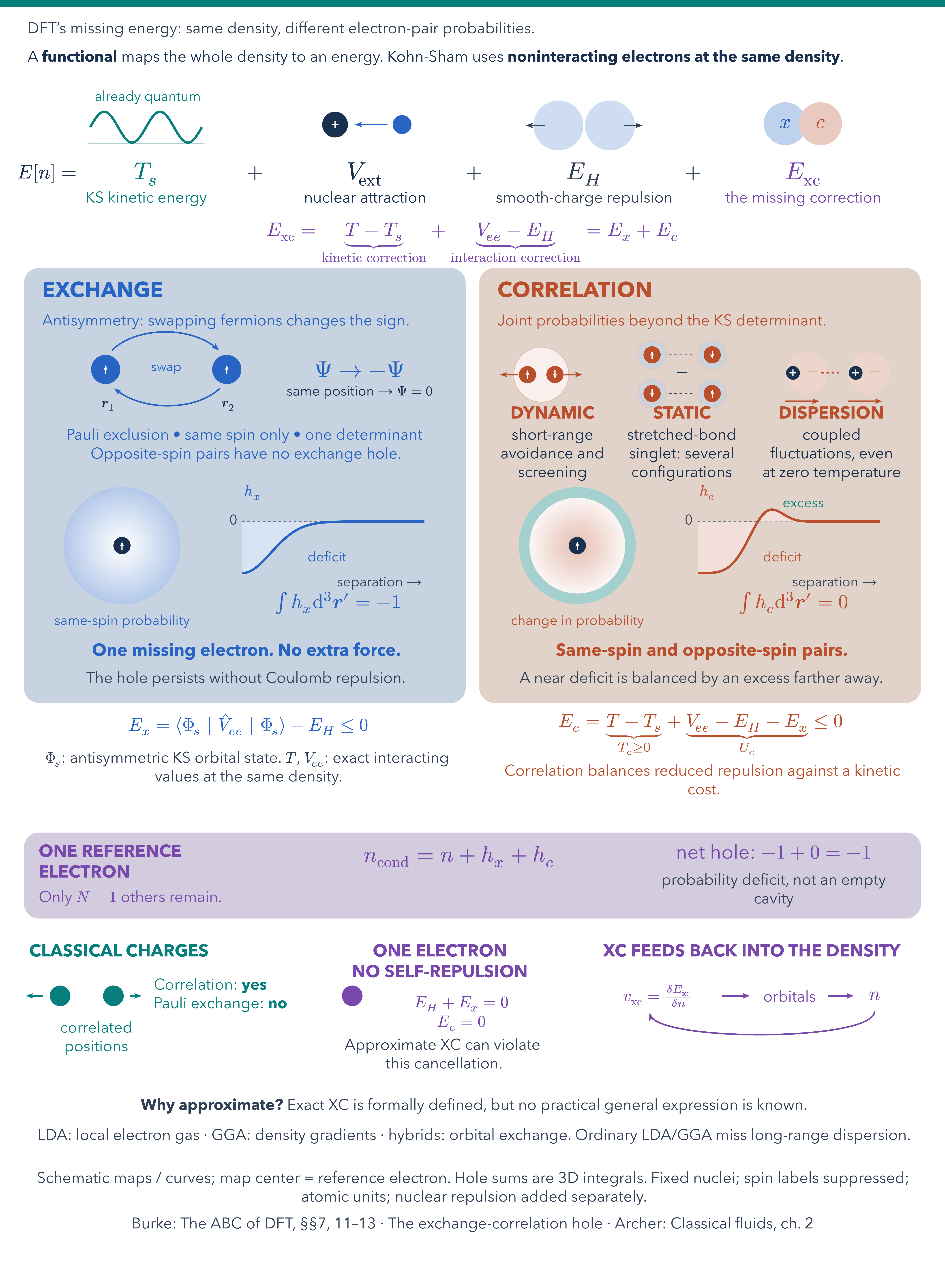
A visual explanation of exchange and correlation in Kohn-Sham density functional theory. Physical icons introduce the four energy terms, a fermion-swap sketch explains exchange antisymmetry, and probability maps and hole profiles show the exchange deficit and correlation redistribution. Three small diagrams illustrate dynamic avoidance, static correlation in a stretched-bond singlet, and dispersion from coupled fluctuations. Compact equations retain the kinetic correlation correction, exact hole sum rules, and one-electron self-interaction cancellation. A classical-charge comparison distinguishes quantum exchange from classical correlation, while a feedback loop connects the XC functional derivative to orbitals and density.
Download
Code
xc-functional.typ (468 lines)
#import "@preview/cetz:0.5.2": canvas, draw
#import draw: bezier, circle, content, line, rect, translate

// Ground-state, nonrelativistic Coulomb DFT, atomic units, integer KS occupations.
// At a fixed density: Exc = T - Ts + Vee - EH; Ex = <Phi_s|Vee|Phi_s> - EH.
// Ec = Tc + Uc, with Tc = T - Ts and Uc = Vee - EH - Ex.
// A physical XC hole gives the interaction correction only; its coupling-strength
// average at fixed density also incorporates Tc in the Coulomb energy integral.
// The schematic profiles below are illustrations, not calculated electron densities.
// Sources: https://dft.uci.edu/teaching/lausanne/ABCDFT.pdf (chapters 7, 11-13),
// https://dft.uci.edu/pubs/B97.pdf (XC holes),
// https://www.bristol.ac.uk/physics/media/theory-theses/archer-aj-thesis.pdf (chapter 2).
#set page(width: auto, height: auto, margin: 0pt, fill: none)
#set text(font: "Avenir Next", size: 18pt, fill: rgb("#22334B"))
#set par(leading: 0.5em)
#set math.equation(numbering: none)

#let ink = rgb("#19304E")
#let muted = rgb("#344257")
#let blue = rgb("#2764C3")
#let orange = rgb("#B94F2C")
#let purple = rgb("#7948AD")
#let teal = rgb("#087F7C")
#let pale_blue = rgb("#c8d3e2")
#let pale_orange = rgb("#e1d3c9")

#let label(left, top, width, body, size: 16pt, color: ink, weight: "regular", centered: false) = {
  content(
    (left, -top),
    block(width: width * 1pt)[
      #text(size: size, fill: color, weight: weight, if centered { align(center, body) } else {
        body
      })
    ],
    anchor: "north-west",
    padding: 0pt,
  )
}
// Use the rendered glyph bounds rather than a top-aligned paragraph for symbols.
#let centered_symbol(center_x, center_y, body, size: 24pt, color: ink) = {
  content(
    (center_x, -center_y),
    text(size: size, fill: color, top-edge: "bounds", bottom-edge: "bounds", body),
    anchor: "center",
    padding: 0pt,
  )
}
#let panel(left, top, width, height, fill) = {
  rect((left, -top), (left + width, -top - height), radius: 17, fill: fill, stroke: none)
}
#let connect(start, end, color: muted) = {
  line(
    start,
    end,
    stroke: 1.8pt + color,
    mark: (end: "stealth", scale: 0.7, fill: color),
  )
}
#let curve(start, end, control_a, control_b, color: muted) = {
  bezier(start, end, control_a, control_b, stroke: 1.8pt + color, mark: (
    end: "stealth",
    scale: 0.7,
    fill: color,
  ))
}
#let electron(center_x, center_y, spin: none, color: blue, radius: 10) = {
  circle((center_x, -center_y), radius: radius, fill: color, stroke: none)
  if spin != none {
    let direction = if spin == "up" { 1 } else { -1 }
    line(
      (center_x, -center_y - direction * 5),
      (center_x, -center_y + direction * 5),
      stroke: 1.3pt + white,
      mark: (end: "stealth", scale: 0.45, fill: white),
    )
  }
}
#let nucleus(center_x, center_y, radius: 9) = {
  circle((center_x, -center_y), radius: radius, fill: ink, stroke: none)
  line((center_x - 4, -center_y), (center_x + 4, -center_y), stroke: 1.3pt + white)
  line((center_x, -center_y - 4), (center_x, -center_y + 4), stroke: 1.3pt + white)
}

// A shaded probability map: the central dot is conditioned on, not a moving particle.
#let density_map(center_x, center_y, radius: 68, kind: "exchange", color: blue) = {
  if kind == "exchange" {
    circle((center_x, -center_y), radius: radius, fill: color.lighten(65%), stroke: none)
    for idx in range(32) {
      let ring_radius = radius * (1 - idx / 34)
      let lightness = 65% + idx / 31 * 33%
      circle(
        (center_x, -center_y),
        radius: ring_radius,
        fill: color.lighten(lightness),
        stroke: none,
      )
    }
  } else if kind == "correlation" {
    circle((center_x, -center_y), radius: radius, fill: teal.lighten(63%), stroke: none)
    for idx in range(28) {
      circle(
        (center_x, -center_y),
        radius: radius * (0.82 - idx / 38),
        fill: orange.lighten(94% - idx / 27 * 27%),
        stroke: none,
      )
    }
  }
  electron(center_x, center_y, spin: "up", color: ink, radius: 10)
}
#let hole_plot(left, top, kind, color) = {
  let baseline = top + 30
  let plot_width = 212
  line((left, -baseline), (left + plot_width, -baseline), stroke: (
    paint: muted,
    thickness: 0.7pt,
    dash: "dashed",
  ))
  let points = range(151).map(idx => {
    let distance = idx / 150 * 4.5
    let value = if kind == "exchange" {
      -calc.exp(-distance * distance)
    } else {
      let scaled_distance = distance / 1.6
      (4 / 3 * calc.pow(scaled_distance, 4) - 1) * calc.exp(-calc.pow(scaled_distance, 4))
    }
    (left + idx / 150 * plot_width, -baseline + 60 * value)
  })
  line(
    (left, -baseline),
    ..points,
    (left + plot_width, -baseline),
    close: true,
    fill: color.lighten(82%),
    stroke: none,
  )
  line(..points, stroke: 2.8pt + color)
  label(
    left + 2,
    top - 12,
    70,
    if kind == "exchange" { [$h_x$] } else { [$h_c$] },
    size: 18pt,
    color: color,
  )
  label(left - 15, baseline - 8, 13, [0], size: 16pt, color: muted)
  label(left + 110, top + 94, 110, [separation →], size: 16pt, color: muted)
  label(left + 76, top + 65, 75, [deficit], size: 16pt, color: color)
  if kind == "correlation" { label(left + 99, top + 2, 90, [excess], size: 16pt, color: teal) }
}

#let centered_label = label.with(centered: true)

#canvas(length: 1pt, {
  rect((0, -51), (1100, -1550), fill: none, stroke: none)
  rect((0, -51), (1100, -59), fill: teal, stroke: none)
  label(
    32,
    77,
    1040,
    [DFT’s missing energy: same density, different electron-pair probabilities.],
    size: 18pt,
    color: muted,
  )

  label(
    32,
    110,
    1036,
    [A *functional* maps the whole density to an energy. Kohn-Sham uses *noninteracting electrons at the same density*.],
    size: 18pt,
  )
  translate((0, -40))

  // === The four terms, drawn as physical ingredients ===
  for (center_x, title, caption, color) in (
    (170, [$T_s$], [KS kinetic energy], teal),
    (425, [$V_"ext"$], [nuclear attraction], ink),
    (680, [$E_H$], [smooth-charge repulsion], muted),
    (935, [$E_"xc"$], [the missing correction], purple),
  ) {
    label(center_x - 100, 200, 200, title, size: 29pt, color: color, centered: true)
    label(center_x - 115, 234, 230, caption, size: 18pt, color: color, centered: true)
  }
  // Orbital wave: Ts is already quantum.
  line((103, -178), (237, -178), stroke: 0.7pt + teal.lighten(65%))
  let wave_points = range(101).map(idx => (
    105 + idx * 1.3,
    -159 + 18 * calc.sin(idx / 100 * 4 * calc.pi),
  ))
  line(..wave_points, stroke: 2.8pt + teal)
  label(107, 117, 130, [already quantum], size: 16pt, color: teal, centered: true)
  // Electron-nucleus attraction.
  nucleus(390, 156, radius: 15)
  electron(468, 156, radius: 11)
  connect((451, -156), (413, -156), color: blue)
  // Hartree: two smooth patches of the same density, no conditional hole.
  circle((650, -157), radius: 29, fill: blue.lighten(78%), stroke: none)
  circle((710, -157), radius: 29, fill: blue.lighten(78%), stroke: none)
  connect((634, -157), (612, -157), color: muted)
  connect((726, -157), (748, -157), color: muted)
  // XC split, indicated with the same colors used below.
  circle((914, -155), radius: 25, fill: blue.lighten(70%), stroke: none)
  circle((955, -155), radius: 25, fill: orange.lighten(70%), stroke: none)
  centered_symbol(914, 155, [$x$], color: blue)
  centered_symbol(955, 155, [$c$], color: orange)
  label(20, 203, 89, [$E[n] =$], size: 23pt)
  for center_x in (297, 552, 807) { label(center_x - 10, 202, 28, [$+$], size: 25pt, color: muted) }
  centered_label(
    30,
    270,
    1040,
    [$E_"xc" = underbrace(T - T_s, "kinetic correction") + underbrace(V_(e e) - E_H, "interaction correction") = E_x + E_c$],
    size: 23pt,
    color: purple,
  )

  // === Exchange: swapping amplitudes and the same-spin hole ===
  panel(28, 323, 514, 506, pale_blue)
  panel(558, 323, 514, 506, pale_orange)
  label(49, 339, 468, [EXCHANGE], size: 25pt, color: blue, weight: "bold")
  label(
    49,
    377,
    468,
    [Antisymmetry: swapping fermions changes the sign.],
    size: 18pt,
    color: blue,
  )

  electron(123, 441, spin: "up", radius: 17)
  electron(264, 441, spin: "up", radius: 17)
  curve((130, -419), (255, -419), (159, -390), (226, -390), color: blue)
  curve((256, -463), (133, -463), (227, -490), (164, -490), color: blue)
  centered_symbol(193.5, 441, [swap], size: 15pt, color: blue)
  label(100, 474, 51, [$bold(r)_1$], size: 16pt, centered: true)
  label(240, 474, 51, [$bold(r)_2$], size: 16pt, centered: true)
  centered_symbol(418.5, 441, [$Psi -> -Psi$], size: 27pt, color: blue)
  label(328, 460, 181, [same position → $Psi = 0$], size: 16pt, centered: true)
  centered_label(
    56,
    510,
    457,
    [Pauli exclusion • same spin only • one determinant],
    size: 18pt,
    color: blue,
  )

  centered_label(
    63,
    532,
    443,
    [Opposite-spin pairs have no exchange hole.],
    size: 18pt,
    color: blue,
  )

  // Both holes use the same map, integral, and summary layout.
  let hole_summary(offset, kind, color, probability, integral, summary, footer) = {
    density_map(142 + offset, 646, kind: kind, color: color)
    label(59 + offset, 727, 166, probability, size: 16pt, color: color, centered: true)
    hole_plot(282 + offset, 588, kind, color)
    label(270 + offset, 703, 247, integral, size: 23pt, color: color, centered: true)
    label(63 + offset, 760, 443, summary, size: 20pt, weight: "bold", color: color, centered: true)
    label(63 + offset, 793, 443, footer, size: 18pt, color: muted, centered: true)
  }
  hole_summary(
    0,
    "exchange",
    blue,
    [same-spin probability],
    [$integral h_x dif^3 bold(r)' = -1$],
    [One missing electron. No extra force.],
    [The hole persists without Coulomb repulsion.],
  )

  // === Correlation: three recognizable physical mechanisms ===
  label(579, 339, 468, [CORRELATION], size: 25pt, color: orange, weight: "bold")
  label(
    579,
    377,
    468,
    [Joint probabilities beyond the KS determinant.],
    size: 18pt,
    color: orange,
  )
  // Dynamic correlation: spatial avoidance.
  circle((630, -447), radius: 32, fill: orange.lighten(91%), stroke: 0.8pt + orange.lighten(60%))
  electron(614, 447, spin: "up", color: orange)
  electron(646, 447, spin: "down", color: orange)
  connect((603, -447), (582, -447), color: orange)
  connect((657, -447), (678, -447), color: orange)
  label(573, 484, 140, [DYNAMIC], size: 20pt, weight: "bold", color: orange, centered: true)
  label(554, 510, 178, [short-range\ avoidance and\ screening], size: 18pt, centered: true)

  // Static correlation: the two separated-atom spin configurations of a singlet.
  for (row_y, first_spin, second_spin) in ((424, "up", "down"), (469, "down", "up")) {
    circle((759, -row_y), radius: 17, fill: rgb("#cdd3da"), stroke: 0.8pt + orange.lighten(65%))
    circle((829, -row_y), radius: 17, fill: rgb("#cdd3da"), stroke: 0.8pt + orange.lighten(65%))
    line((779, -row_y), (809, -row_y), stroke: (paint: muted, thickness: 0.8pt, dash: "dashed"))
    electron(759, row_y, spin: first_spin, color: orange, radius: 10)
    electron(829, row_y, spin: second_spin, color: orange, radius: 10)
  }
  centered_symbol(794, 447, [$-$], size: 19pt)
  label(724, 484, 140, [STATIC], size: 20pt, weight: "bold", color: orange, centered: true)
  centered_label(
    718,
    510,
    151,
    [stretched-bond\ singlet: several\ configurations],
    size: 18pt,
  )

  // Dispersion: correlated instantaneous dipoles, not permanent ones.
  for center_x in (931, 1004) {
    circle((center_x + 8, -445), radius: 24, fill: orange.lighten(76%), stroke: none)
    nucleus(center_x - 8, 445, radius: 8)
    centered_symbol(center_x + 14, 445, [$-$], size: 18pt, color: orange)
    connect((center_x - 17, -478), (center_x + 23, -478), color: orange)
  }
  line((956, -445), (978, -445), stroke: (paint: orange, thickness: 1.4pt, dash: "dashed"))
  label(890, 484, 155, [DISPERSION], size: 20pt, weight: "bold", color: orange, centered: true)
  centered_label(
    883,
    510,
    170,
    [coupled\ fluctuations, even\ at zero temperature],
    size: 18pt,
  )

  hole_summary(
    530,
    "correlation",
    orange,
    [change in probability],
    [$integral h_c dif^3 bold(r)' = 0$],
    [Same-spin and opposite-spin pairs.],
    [A near deficit is balanced by an excess farther away.],
  )

  // === Compact energy ledger: preserve the kinetic correction ===
  centered_label(
    47,
    847,
    484,
    [$E_x = chevron.l Phi_s bar.v hat(V)_(e e) bar.v Phi_s chevron.r - E_H <= 0$],
    size: 21pt,
    color: blue,
  )
  centered_label(
    577,
    842,
    477,
    [$E_c = underbrace(T - T_s, T_c >= 0) + underbrace(V_(e e) - E_H - E_x, U_c) <= 0$],
    size: 22pt,
    color: orange,
  )
  centered_label(
    45,
    886,
    485,
    [$Phi_s$: antisymmetric KS orbital state. $T$, $V_(e e)$: exact interacting values at the same density.],
    size: 18pt,
    color: muted,
  )
  centered_label(
    580,
    901,
    475,
    [Correlation balances reduced repulsion against a kinetic cost.],
    size: 18pt,
    color: orange,
  )

  // === The sum rule: the picture to remember ===
  panel(28, 980, 1044, 100, rgb("#d2ccde"))
  label(45, 994, 275, [ONE REFERENCE ELECTRON], size: 20pt, color: purple, weight: "bold")
  label(45, 1048, 275, [Only $N - 1$ others remain.], size: 18pt, color: purple)
  label(336, 996, 397, [$n_"cond" = n + h_x + h_c$], size: 26pt, color: purple, centered: true)
  label(758, 994, 285, [net hole: $-1 + 0 = -1$], size: 23pt, color: purple, centered: true)
  centered_label(
    758,
    1028,
    285,
    [probability deficit, not an empty cavity],
    size: 18pt,
    color: muted,
  )

  // === Classical contrast, exact one-electron check, and the KS feedback loop ===
  label(34, 1110, 310, [CLASSICAL CHARGES], size: 20pt, color: teal, weight: "bold")
  electron(70, 1170, color: teal, radius: 12)
  electron(132, 1170, color: teal, radius: 12)
  connect((50, -1170), (30, -1170), color: teal)
  connect((151, -1170), (165, -1170), color: teal)
  label(36, 1200, 152, [correlated positions], size: 18pt, color: teal, centered: true)
  label(179, 1150, 172, [Correlation: *yes*\ Pauli exchange: *no*], size: 18pt, color: teal)

  centered_label(
    383,
    1110,
    258,
    [ONE ELECTRON\ NO SELF-REPULSION],
    size: 20pt,
    color: purple,
    weight: "bold",
  )
  electron(410, 1170, color: purple, radius: 12)
  centered_label(
    385,
    1220,
    260,
    [Approximate XC can violate this cancellation.],
    size: 18pt,
    color: muted,
  )
  label(435, 1170, 204, [$E_H + E_x = 0$\ $E_c = 0$], size: 19pt, color: purple, centered: true)

  centered_label(
    700,
    1110,
    350,
    [XC FEEDS BACK INTO THE DENSITY],
    size: 20pt,
    color: purple,
    weight: "bold",
  )
  centered_symbol(765.5, 1170, [$v_"xc" = (delta E_"xc") / (delta n)$], size: 19pt, color: purple)
  connect((840, -1170), (873, -1170), color: purple)
  centered_symbol(919, 1170, [orbitals], size: 18pt, color: purple)
  connect((964, -1170), (994, -1170), color: purple)
  centered_symbol(1018, 1170, [$n$], size: 22pt, color: purple)
  curve((1018, -1188), (756, -1190), (1018, -1224), (756, -1224), color: purple)

  centered_label(
    30,
    1290,
    1040,
    [*Why approximate?* Exact XC is formally defined, but no practical general expression is known.],
    size: 18pt,
    color: muted,
  )
  centered_label(
    30,
    1325,
    1040,
    [LDA: local electron gas · GGA: density gradients · hybrids: orbital exchange. Ordinary LDA/GGA miss long-range dispersion.],
    size: 18pt,
    color: muted,
  )
  centered_label(
    30,
    1375,
    1040,
    [Schematic maps / curves; map center = reference electron. Hole sums are 3D integrals. Fixed nuclei; spin labels suppressed; atomic units; nuclear repulsion added separately.],
    size: 18pt,
    color: muted,
  )
  centered_label(
    30,
    1428,
    1040,
    [#link("https://dft.uci.edu/teaching/lausanne/ABCDFT.pdf")[Burke: The ABC of DFT, §§7, 11–13] · #link("https://dft.uci.edu/pubs/B97.pdf")[The exchange-correlation hole] · #link("https://www.bristol.ac.uk/physics/media/theory-theses/archer-aj-thesis.pdf")[Archer: Classical fluids, ch. 2]],
    size: 18pt,
    color: muted,
  )
})