Convex Functions

mathcetztikz

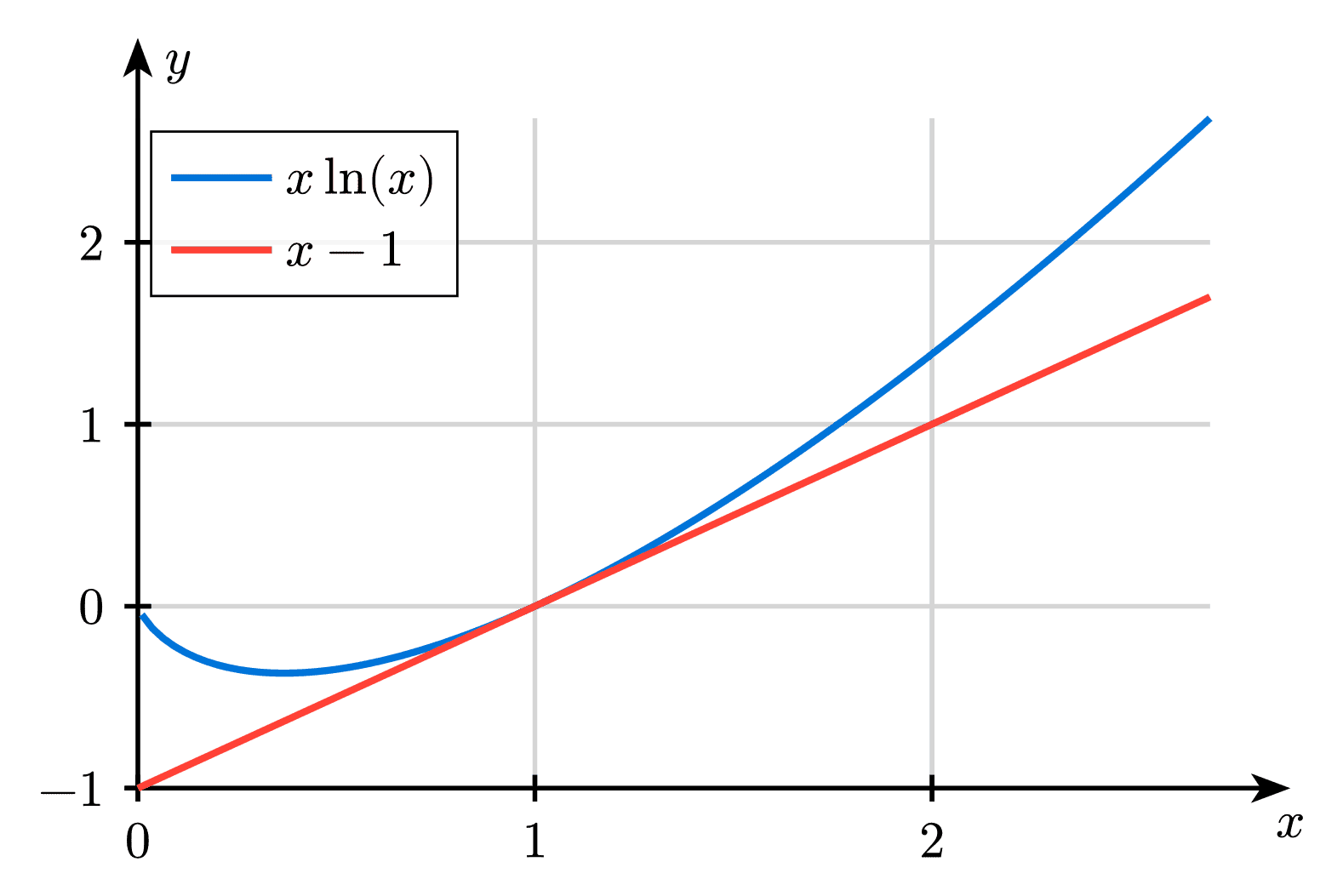
$x$ and $-x\log(x)$ are concave functions. Since $\ln(p)$ decomposes into sums of these two components, it too must be concave. Any extremum of a concave function is a maximum. This fact is used in statistical physics to find the equilibrium distribution of many-particle systems. See problem 2 on this exercise sheet.

Download

PNG PDF SVG

Code

LaTeX

convex-functions.tex (26 lines)

\documentclass{standalone}

\usepackage{pgfplots}
\pgfplotsset{compat=newest}

\begin{document}
\begin{tikzpicture}
  \begin{axis}[
      domain=0:2.7,
      xlabel=$x$,
      smooth,thick,
      axis lines=center,
      every tick/.style={thick},
      legend style={cells={anchor=west}},
      legend pos=north west]

    \addplot[color=blue]{x*ln(x)};

    \addplot[color=red]{x-1};

    \legend{$x \, \ln(x)$,$x-1$}

  \end{axis}
\end{tikzpicture}
\end{document}

Typst

convex-functions.typ (42 lines)

#import "@preview/cetz:0.3.2": canvas
#import "@preview/cetz-plot:0.1.1": plot

#set page(width: auto, height: auto, margin: 8pt)

#let size = (8, 5)

#canvas({
  plot.plot(
    size: size,
    x-min: 0,
    x-max: 2.7,
    x-label: $x$,
    y-tick-step: 1,
    x-tick-step: 0.5,
    x-grid: true,
    y-grid: true,
    legend: "inner-north-west",
    {
      plot.add-hline(0, style: (stroke: 0.5pt))
      plot.add-vline(0, style: (stroke: 0.5pt))

      // x ln(x) function
      plot.add(
        style: (stroke: blue + 1.5pt),
        domain: (0.01, 2.7), // avoid x=0 since ln(0) is undefined
        samples: 100,
        label: $x ln(x)$,
        x => x * calc.ln(x),
      )

      // x-1 function
      plot.add(
        style: (stroke: red + 1.5pt),
        domain: (0, 2.7),
        label: $x-1$,
        x => x - 1,
      )
    },
  )
})