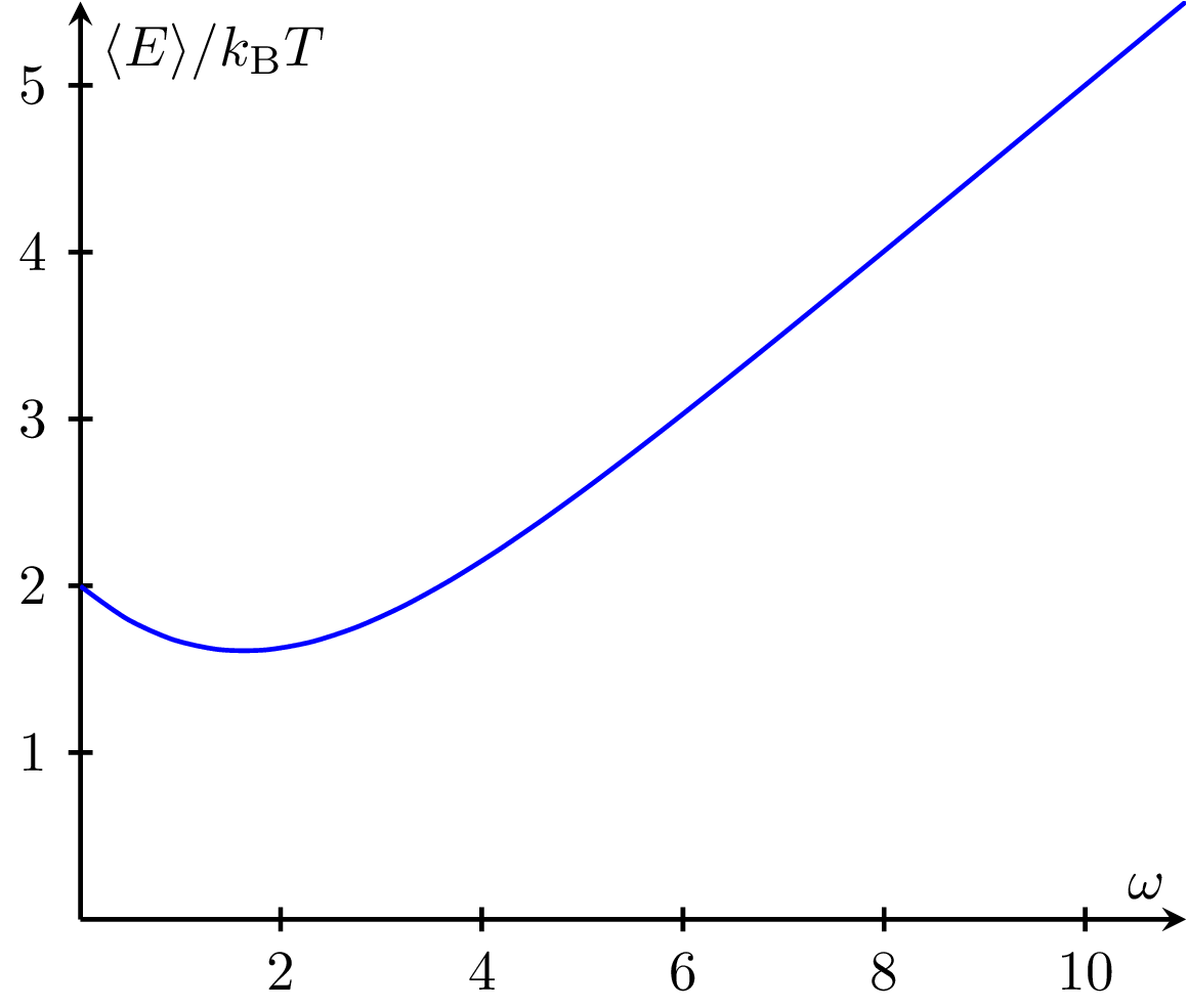
Harmonic oscillator energy vs angular frequency
\documentclass{standalone}
\usepackage{pgfplots,mathtools}
\pgfplotsset{compat=newest}
\begin{document}
\begin{tikzpicture}
\begin{axis}[
xlabel = $\omega = \sqrt{k/m}$,
ylabel = $\langle E\rangle/k_\text{B} T$,
domain = 0.01:11,
ymin = 0,
smooth,thick,
axis lines = center,
every tick/.style = thick]
\def\h{1}
\def\b{1}
\def\eev{1/2*\h*x*(1 + 4/(e^(\b*\h*x) - 1))}
\addplot[color=blue]{\eev};
\end{axis}
\end{tikzpicture}
\end{document}
#import "@preview/cetz:0.3.2": canvas, draw
#import "@preview/cetz-plot:0.1.1": plot
#set page(width: auto, height: auto, margin: 8pt)
#let size = (8, 5)
#canvas({
draw.set-style(
axes: (
y: (label: (anchor: "north-west", offset: -0.2), mark: (end: "stealth", fill: black)),
x: (label: (anchor: "north", offset: 0.1), mark: (end: "stealth", fill: black)),
),
)
plot.plot(
size: size,
x-min: 0,
x-max: 11,
y-min: 0,
x-label: $omega = sqrt(k/m)$,
y-label: $angle.l E angle.r \/ k_"B" T$,
x-tick-step: 2,
y-tick-step: 2,
axis-style: "left",
{
// Define constants from original
let h = 1
let b = 1
// Add the energy expectation value curve
plot.add(
style: (stroke: blue + 1.5pt),
domain: (0.01, 11), // Avoid x=0 due to division
samples: 200, // More samples for smoother curve
x => {
// E = (1/2)hω(1 + 4/(exp(βhω) - 1))
let hw = h * x
let exp_term = calc.exp(b * hw)
(1 / 2) * hw * (1 + 4 / (exp_term - 1))
},
)
},
)
})