QFT Propagator Poles
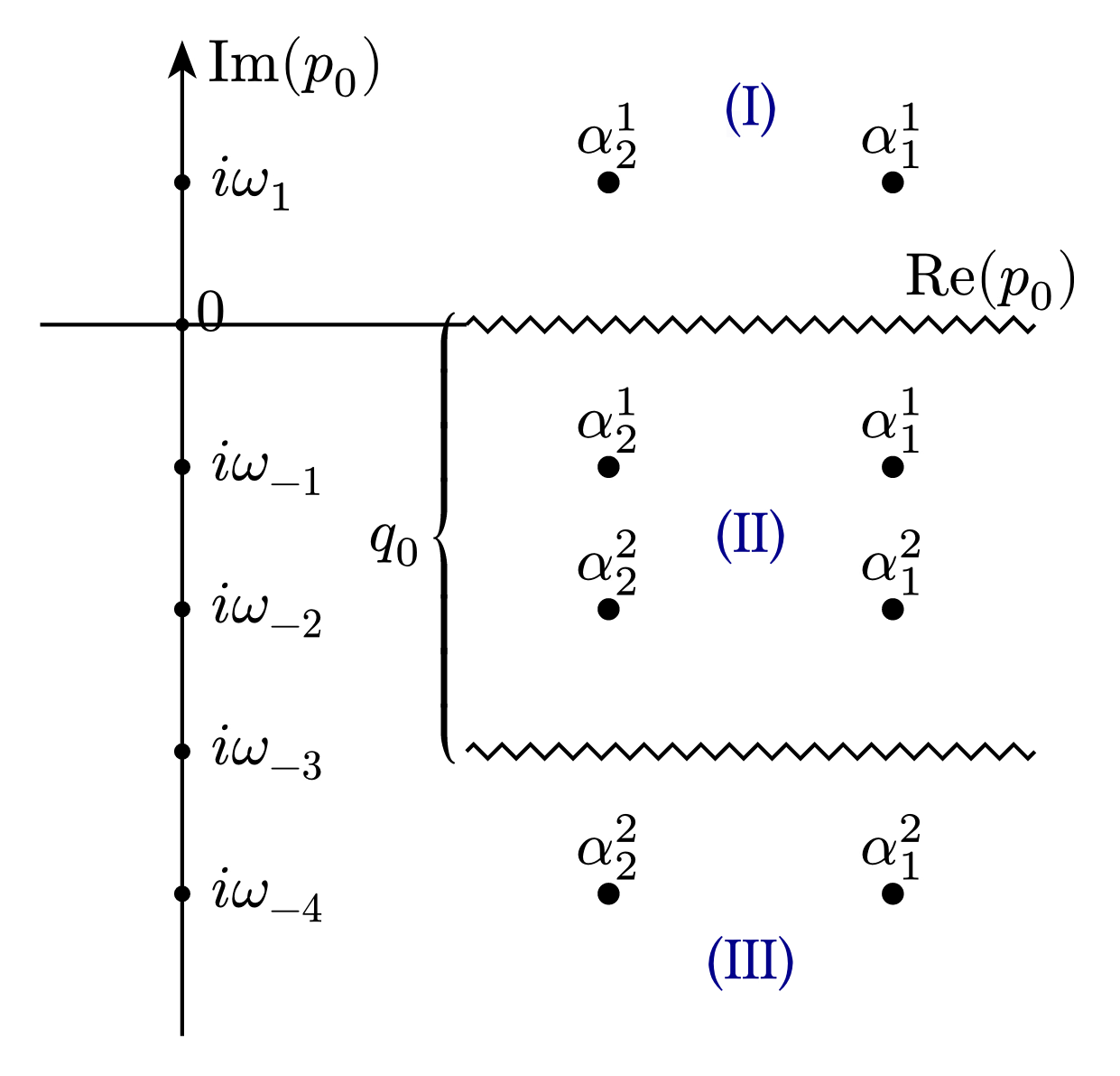
Complex plane visualization of propagator poles and branch cuts in quantum field theory. The diagram shows the analytic structure of Green's functions, including the relationship between retarded/advanced propagators and the placement of poles relative to the real axis. This structure helps understand causality and the connection to Matsubara frequencies.
Download
Code
qft-propagator-poles.typ (90 lines)
#import "@preview/cetz:0.5.2": canvas, decorations, draw
#import draw: circle, content, line

#set page(width: auto, height: auto, margin: 8pt, fill: none)
#set text(size: 12pt)

#canvas({
  let xrange = 6
  let yrange = 4

  // Axes styles
  let arrow-style = (mark: (end: "stealth", fill: black))
  let line-style = (stroke: 0.75pt)
  let zigzag-style = (amplitude: 0.1, segment-length: 0.2)

  // Main axes
  line((-1, 0), (2, 0), ..line-style, name: "x-axis-left")
  decorations.zigzag(
    line((2, 0), (xrange, 0)),
    ..zigzag-style,
    ..line-style,
    name: "x-axis-right",
  )
  content(
    (rel: (-0.3, 0.3), to: "x-axis-right.end"),
    $"Re"(p_0)$,
    name: "x-label",
  )

  decorations.zigzag(
    line((2, -3), (xrange, -3), name: "lower-zigzag"),
    ..zigzag-style,
    ..line-style,
  )

  line((0, -yrange - 1), (0, 2), ..arrow-style, ..line-style, name: "y-axis")
  content((rel: (0.8, -0.2), to: "y-axis.end"), $"Im"(p_0)$, name: "y-label")

  // Brace for q_0
  content(
    (2, -1.5),
    [#math.underbrace(box(width: 7.5em))],
    name: "q0-brace",
    angle: -90deg,
  )
  content((rel: (-0.5, 0), to: "q0-brace"), $q_0$, name: "q0-label")

  // Matsubara frequencies
  for n in range(-yrange, 2) {
    if n != 0 {
      circle((0, n), radius: 0.04, fill: black, name: "matsubara-" + str(n))
      content("matsubara-" + str(n), $i omega_#n$, anchor: "west", padding: 0.2)
    }
  }
  circle((0, 0), radius: 0.03, fill: black, name: "origin")
  content((0.2, 0.1), $0$, name: "origin-label")

  // Poles
  let pole(x, y, label) = {
    circle(
      (x, y),
      radius: 0.06,
      fill: black,
      name: "pole-" + str(x) + "-" + str(y),
    )
    content(
      "pole-" + str(x) + "-" + str(y),
      label,
      anchor: "south",
      padding: 0.1,
    )
  }

  for (y-pos, left-label, right-label) in (
    (1, $alpha_2^1$, $alpha_1^1$),
    (-1, $alpha_2^1$, $alpha_1^1$),
    (-2, $alpha_2^2$, $alpha_1^2$),
    (-4, $alpha_2^2$, $alpha_1^2$),
  ) {
    pole(3, y-pos, left-label)
    pole(5, y-pos, right-label)
  }

  // Region labels
  let blue = rgb("#00008B") // DarkBlue equivalent
  for (idx, y-pos, label) in ((1, 1.5, [(I)]), (2, -1.5, [(II)]), (3, -4.5, [(III)])) {
    content((4, y-pos), text(fill: blue, label), name: "region-" + str(idx))
  }
})