« home

Cost vs Accuracy in Quantum Mechanical Simulations

physicsquantum mechanicssolid state physicsdensity functional theorycetztikz

Cost vs accuracy trade-off for different quantum mechanics approximations. NN denotes the system size, usually the number of electrons. Source: Frank Noe.
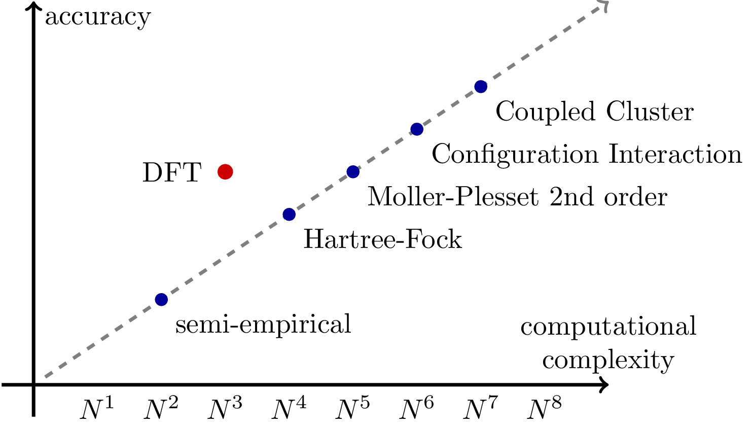

Cost vs Accuracy in Quantum Mechanical Simulations

  Download

PNGPDFSVG

  Code

  LaTeX

qm-cost-vs-acc.tex (28 lines)

\documentclass[tikz]{standalone}

\def\range{9}
\def\xyRatio{2/3}
\def\circSize{1mm}

\begin{document}
\begin{tikzpicture}[->, very thick, align=center, scale=0.8]

  \draw (0,-0.5) -- (0,\range*\xyRatio) node[below right] {accuracy};
  \draw (-0.5,0) -- (\range,0) node[above] {computational\\complexity};
  \foreach \n in {1,...,8}
  \node[below] at (\n,0) {$N^\n$};

  \draw[dashed, gray, shorten <=5] (0,0) -- (\range,\range*\xyRatio);

  \foreach \n/\name/\abbr in {2/semi-empirical/SE, 4/Hartree-Fock/HF, 5/Moller-Plesset 2nd order/MP2, 6/Configuration Interaction/CISD, 7/Coupled Cluster/CCSD(T)}
  \fill[blue!60!black] (\n,\xyRatio*\n) circle (\circSize)
  node[align=left, below right=1pt, black] (\abbr) {\name};

  % \draw[red, thick] (HF) -- (SE);

  \fill[red!80!black] (3,5*\xyRatio) circle (1.2*\circSize) node[left=1ex, black] {DFT};
  % \fill[blue!60!black] (4.5,6.5*\xyRatio) circle (\circSize) node[left=1ex, black] {Deep QMC};

\end{tikzpicture}
\end{document}

  Typst

qm-cost-vs-acc.typ (82 lines)

#import "@preview/cetz:0.3.2": canvas, draw

#set page(width: auto, height: auto, margin: 8pt)

#let range = 9
#let xy-ratio = 2 / 3

#canvas({
  import draw: line, content, circle

  let arrow-style = (mark: (end: "stealth", scale: .75), stroke: black + 1pt, fill: black)

  // Draw axes
  line((-0.5, 0), (range, 0), ..arrow-style) // x-axis
  line((0, -0.5), (0, range * xy-ratio), ..arrow-style) // y-axis

  // Add axis labels
  content(
    (range + 0.1, .15),
    [computational complexity],
    anchor: "south-east",
  )
  content(
    (0.2, range * xy-ratio),
    [accuracy],
    anchor: "north-west",
  )

  // Add N^n labels below x-axis
  for n in std.range(1, 9) {
    content(
      (n, -0.3),
      $N^#n$,
      anchor: "north",
    )
  }

  // Add dashed diagonal line
  line(
    (0, 0),
    (range, range * xy-ratio),
    stroke: (dash: "dashed", paint: gray, thickness: .75pt),
  )

  // Data points with labels
  let methods = (
    (2, "semi-empirical", "SE"),
    (4, "Hartree-Fock", "HF"),
    (5, "Moller-Plesset 2nd order", "MP2"),
    (6, "Configuration Interaction", "CISD"),
    (7, "Coupled Cluster", "CCSD(T)"),
  )

  // Draw blue dots for standard methods
  for (x, name, abbr) in methods {
    circle(
      (x, x * xy-ratio),
      radius: 2pt,
      fill: rgb("#393998"),
      stroke: none,
    )
    content(
      (x + 0.2, x * xy-ratio - 0.2),
      [#name],
      anchor: "north-west",
    )
  }

  // Special point for DFT
  circle(
    (3, 5 * xy-ratio),
    radius: 2.4pt,
    fill: rgb("#de2626"),
    stroke: none,
  )
  content(
    (2.7, 5 * xy-ratio),
    [DFT],
    anchor: "east",
  )
})