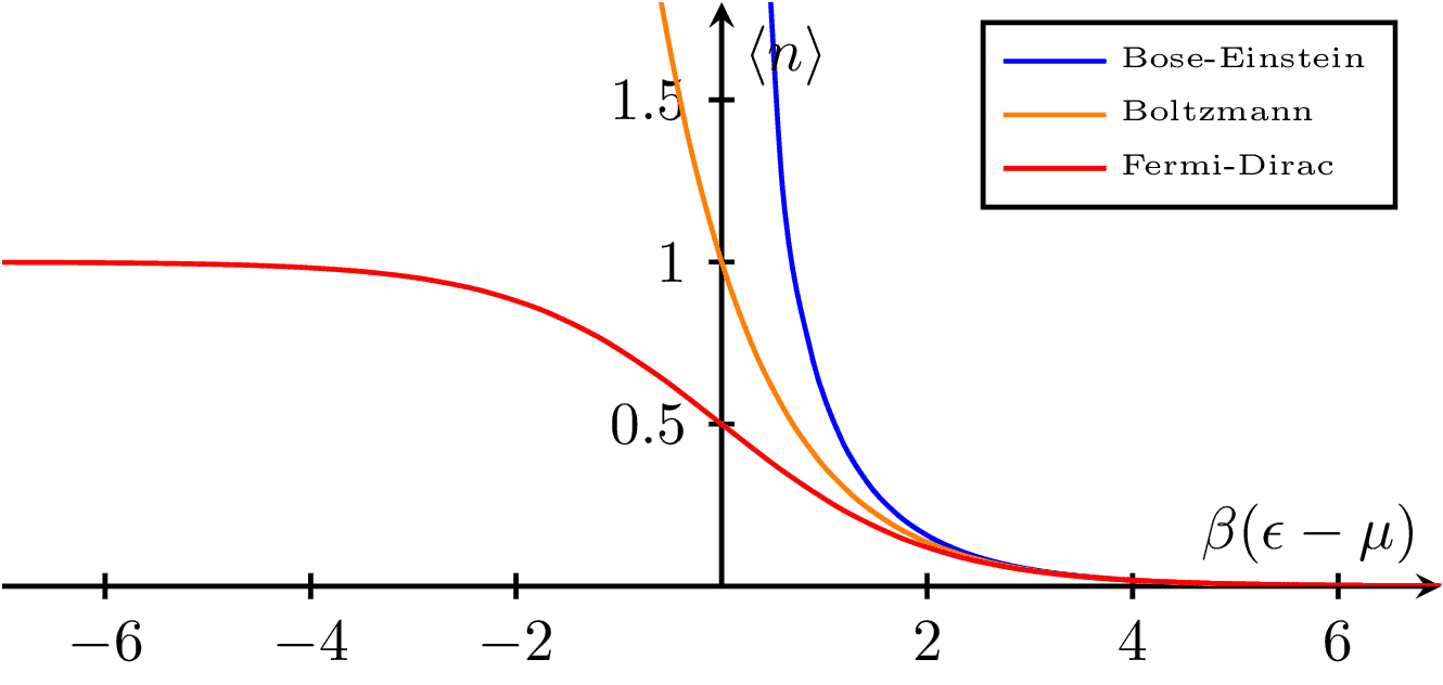
A plot comparing the identical particle distribution functions of Bose-Einstein, Boltzmann, and Fermi-Dirac statistics as a function of the reduced chemical potential . This visualization highlights the differences between the three types of distribution functions, which are used to describe the behavior of particles in different statistical systems.
\documentclass{standalone}
\usepackage{pgfplots}
\pgfplotsset{compat=newest}
\begin{document}
\begin{tikzpicture}
\begin{axis}[
xlabel = $\beta (\epsilon - \mu)$,
ylabel = $\langle n\rangle$,
ymin = 0,ymax = 1.8,
smooth,thick,
axis lines = center,
every tick/.style = {thick},
legend cell align=left,
legend style={legend pos=north east,font=\tiny},
width=10cm,height=5cm]
\def\xmax{7}
\addplot[color=blue,domain=0:\xmax]{1/(e^x - 1)};
\addplot[color=orange,domain=-1:\xmax]{1/e^x};
\addplot[color=red,domain = -\xmax:\xmax]{1/(e^x + 1)};
\legend{Bose-Einstein,Boltzmann,Fermi-Dirac}
\end{axis}
\end{tikzpicture}
\end{document}
#import "@preview/cetz:0.3.2": canvas, draw
#import "@preview/cetz-plot:0.1.1": plot
#set page(width: auto, height: auto, margin: 8pt)
// Distribution functions
#let bose-einstein(x) = 1 / (calc.exp(x) - 1)
#let boltzmann(x) = 1 / calc.exp(x)
#let fermi-dirac(x) = 1 / (calc.exp(x) + 1)
#canvas({
draw.set-style(
axes: (
y: (mark: (end: "stealth", fill: black), label: (anchor: "north-west", offset: -0.2)),
x: (mark: (end: "stealth", fill: black), label: (anchor: "south-east", offset: -0.2)),
),
)
plot.plot(
size: (8, 5),
x-label: $beta (epsilon - mu)$,
y-label: $angle.l n angle.r$,
x-min: -7,
x-max: 7,
y-min: 0,
y-max: 1.8,
x-tick-step: 2,
y-tick-step: 0.5,
axis-style: "school-book",
x-grid: true,
y-grid: true,
legend: "inner-north-east",
legend-style: (stroke: 0.5pt, scale: 80%),
{
// Bose-Einstein distribution
plot.add(
style: (stroke: blue + 1.5pt),
domain: (0.1, 7), // Avoid x=0 since BE diverges there
samples: 200,
label: "Bose-Einstein",
bose-einstein,
)
// Boltzmann distribution
plot.add(
style: (stroke: orange + 1.5pt),
domain: (-1, 7),
samples: 100,
label: "Boltzmann",
boltzmann,
)
// Fermi-Dirac distribution
plot.add(
style: (stroke: red + 1.5pt),
domain: (-7, 7),
samples: 100,
label: "Fermi-Dirac",
fermi-dirac,
)
},
)
})