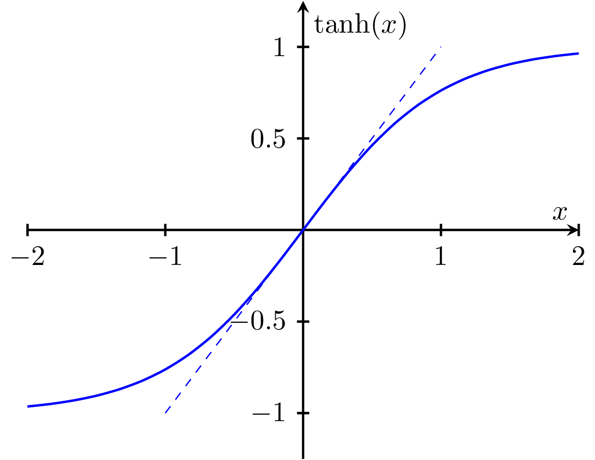
Plot of the hyperbolic tangent. tanh(x) goes to +/- 1 for x to +- infinity while it is approximately linear for abs(x) < 1. Appears in many places in physics, e.g. in the magnetization of an ideal paramagnet of independent spins.
\documentclass{standalone}
\usepackage{pgfplots}
\pgfplotsset{compat=newest}
\begin{document}
\begin{tikzpicture}
\begin{axis}[
xlabel = $x$,
ylabel = $\tanh(x)$,
ymin = -1.25,ymax = 1.25,
domain = -2:2,
smooth,thick,
axis lines = center,
every tick/.style = {thick}]
\addplot[color=blue]{tanh(x)};
\addplot[color=blue,dashed,domain=-1:1,thin]{x};
\end{axis}
\end{tikzpicture}
\end{document}
#import "@preview/cetz:0.3.2": canvas, draw
#import "@preview/cetz-plot:0.1.1": plot
#set page(width: auto, height: auto, margin: 5pt)
#canvas({
draw.set-style(
axes: (
y: (mark: (end: "stealth", fill: black), label: (anchor: "north-west", offset: -0.2)),
x: (mark: (end: "stealth", fill: black), label: (anchor: "south-east", offset: -0.2)),
),
)
plot.plot(
size: (8, 5),
x-label: $x$,
y-label: $tanh(x)$,
y-max: 1.25,
y-min: -1.25,
x-max: 2,
x-min: -2,
x-tick-step: 1,
y-tick-step: 0.5,
axis-style: "school-book",
{
// Main tanh curve
plot.add(
style: (stroke: blue + 1.5pt),
domain: (-2, 2),
samples: 100,
x => calc.tanh(x),
)
// Dashed line y=x from -1 to 1
plot.add(
style: (stroke: (dash: "dashed", paint: blue, thickness: 0.5pt)),
samples: 2,
domain: (-1.4, 1.4),
x => x,
)
},
)
})