DFT Choices
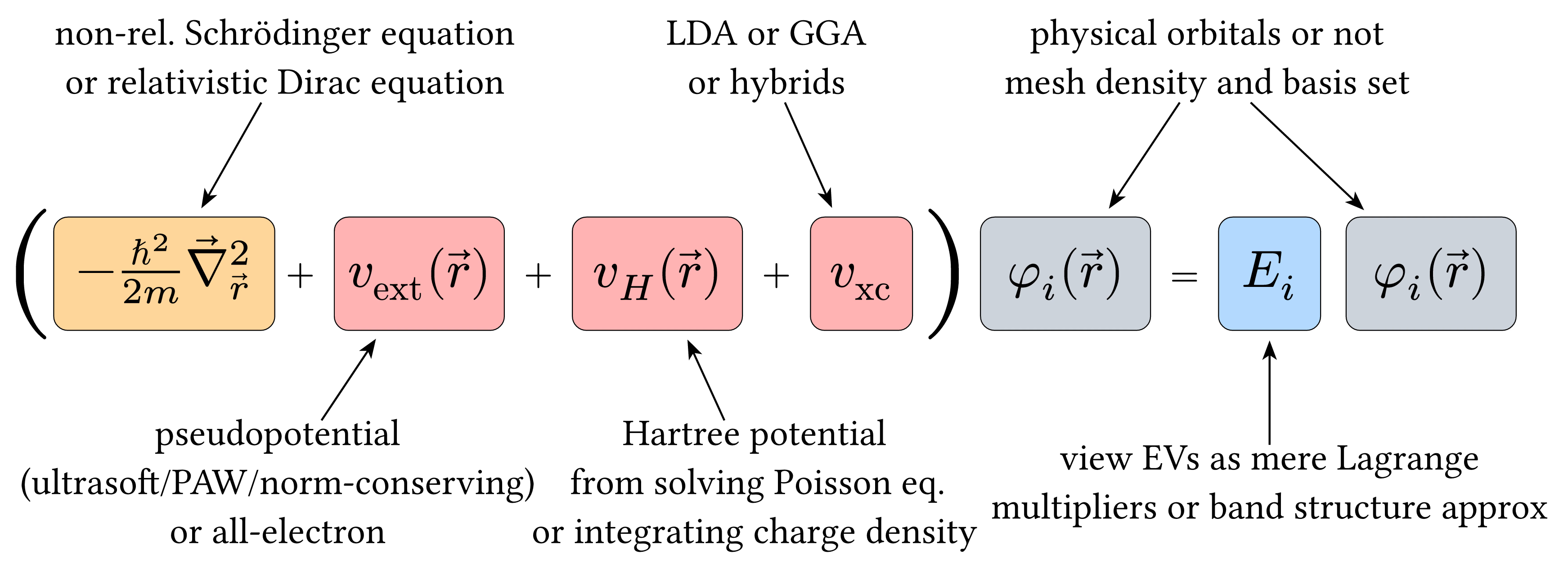
A diagram illustrating the various choices and components in density functional theory (DFT) calculations, including kinetic energy, external potential, Hartree potential, and exchange-correlation terms.
Download
Code
dft-choices.typ (131 lines)
#import "@preview/cetz:0.5.2": canvas, draw
#import draw: content, line, rect

#set page(width: auto, height: auto, margin: 8pt, fill: none)
#set text(size: 15pt)

#canvas({
  let node-sep = 1.7 // Reduced horizontal separation
  let arrow-style = (
    mark: (end: "stealth", fill: black, offset: 4pt),
    stroke: 0.8pt,
  )
  let node-height = 1.6 // Shorter boxes
  let node-width = 1.2 // Increased for larger text

  let node(pos, body, fill: none, name: none, width: node-width, height: node-height) = {
    rect(
      (rel: (-width, -height / 2), to: pos),
      (rel: (2 * width, height)),
      fill: fill,
      stroke: 0.4pt,
      radius: 0.2,
      name: name,
    )
    content(name, scale(140%, body))
  }

  node(
    (0, 0),
    $-frac(planck^2, 2m) arrow(nabla)_(arrow(r))^(2)$,
    fill: rgb("#ffd699"),
    name: "kinetic",
    width: 1.3 * node-width,
  ) // Kinetic term

  content(
    (rel: (-1.6 * node-width, 0.1), to: "kinetic"),
    scale(350%, $($),
    name: "lparen",
  ) // Opening parenthesis

  content((rel: (1.6 * node-width, 0), to: "kinetic"), $+$, name: "plus-1")

  let plus-name = "plus-1"
  for (idx, name, label, offset, width) in (
    (0, "ext", $v_"ext" (arrow(r))$, 1.4, node-width),
    (1, "hartree", $v_H (arrow(r))$, 1.4, node-width),
    (2, "xc", $v_"xc"$, 1, .6 * node-width),
  ) {
    node(
      (rel: (offset * node-width, 0), to: plus-name),
      label,
      fill: rgb("#ffb3b3"),
      name: name,
      width: width,
    )
    if idx < 2 {
      plus-name = "plus-" + str(idx + 2)
      content((rel: (1.4 * node-width, 0), to: name), $+$, name: plus-name)
    }
  }

  content(
    (rel: (1 * node-width, 0.1), to: "xc"),
    scale(350%, $)$),
    name: "rparen",
    padding: 5pt,
  ) // Large closing parenthesis

  node(
    (rel: (2.4 * node-width, 0), to: "xc"),
    $phi_i (arrow(r))$,
    fill: rgb("#cdd3da"),
    name: "phi1",
  ) // Wavefunction 1

  content((rel: (1.4 * node-width, 0), to: "phi1"), $=$, name: "eq-1")

  node(
    (rel: (1 * node-width, 0), to: "eq-1"),
    $E_i$,
    fill: rgb("#b3d9ff"),
    name: "energy",
    width: 0.6 * node-width,
  ) // Energy

  node(
    (rel: (1.9 * node-width, 0), to: "energy"),
    $phi_i (arrow(r))$,
    fill: rgb("#cdd3da"),
    name: "phi2",
  ) // Wavefunction 2

  let comment(pos, body, target) = {
    let name = target + "-comment"
    content(pos, align(center, body), name: name)
    line(name, target, ..arrow-style)
  }

  for spec in (
    (
      (node-sep, 3),
      [non-rel. Schrödinger equation\ or relativistic Dirac equation],
      "kinetic",
    ),
    (
      (rel: (-2, -3), to: "ext"),
      [pseudopotential\ (ultrasoft/PAW/norm-conserving)\ or all-electron],
      "ext",
    ),
    (
      (4.9 * node-sep, -3),
      [Hartree potential\ from solving Poisson eq.\ or integrating charge density],
      "hartree",
    ),
    ((5 * node-sep, 3), [LDA or GGA\ or hybrids], "xc"),
    (
      (rel: (2, 3), to: "phi1"),
      [physical orbitals or not\ mesh density and basis set],
      "phi1",
    ),
  ) { comment(..spec) }
  line("phi1-comment", "phi2", ..arrow-style)

  comment(
    (rel: (0, -3), to: "energy"),
    [view EVs as mere Lagrange\ multipliers or band structure approx],
    "energy",
  )
})