How Atoms Become Energy Bands
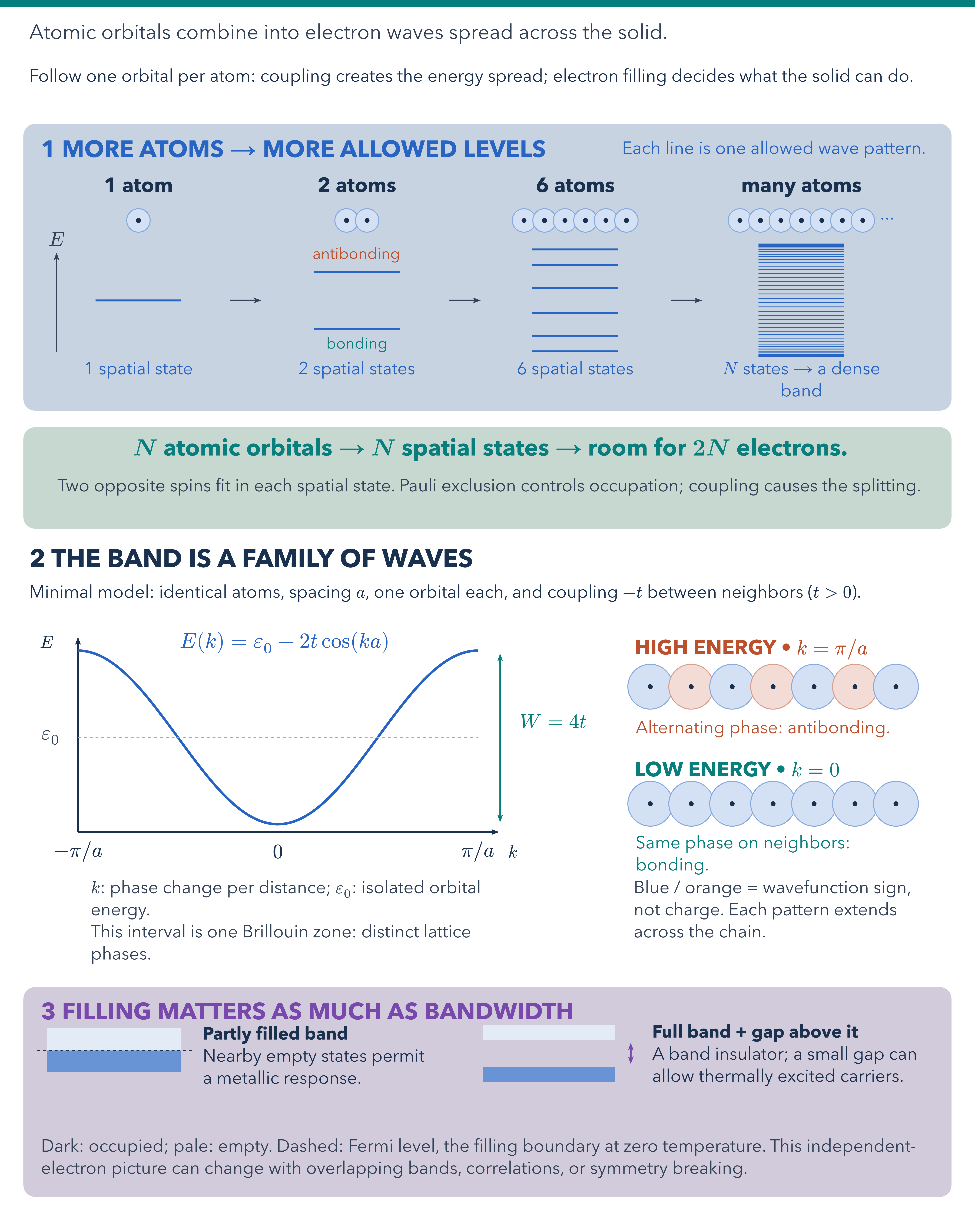
A visual progression from one atomic orbital to a pair, a finite chain, and a dense energy band. Finite-chain levels are calculated from a uniform nearest-neighbor tight-binding model, and the infinite-chain cosine dispersion connects wavefunction phase patterns to bonding, antibonding, and bandwidth. Explicit state and spin counting separates coupling-induced splitting from Pauli filling. Occupation cartoons explain a partially filled band and a filled band separated from empty states by a gap, with the limitations of the independent-electron picture stated explicitly.
Download
Code
how-atoms-become-energy-bands.typ (266 lines)
#import "@preview/cetz:0.5.2": canvas, draw
#import draw: circle, content, line, rect

// One orthonormal orbital per atom, spin-degenerate independent electrons,
// uniform nearest-neighbor hopping H_(j,j+1) = -t with t > 0.
// Open chain: E_m = epsilon_0 - 2t cos(m pi/(N+1)), m = 1,...,N.
// Infinite periodic chain: E(k) = epsilon_0 - 2t cos(ka), bandwidth W = 4t.
// Finite level diagrams use exactly this open-chain spectrum, epsilon_0 = 0, t = 1.
// Sources: MIT OCW 3.23 (2007), lecture 10, Tight-Binding:
// https://ocw.mit.edu/courses/3-23-electrical-optical-and-magnetic-properties-of-materials-fall-2007/resources/lec10/
// Ashcroft & Mermin, Solid State Physics (1976), chapters 10 and 11.
#set page(width: auto, height: auto, margin: 0pt, fill: none)
#set text(font: "Avenir Next", size: 18pt, fill: rgb("#19304E"))
#set par(leading: 0.55em)
#set math.equation(numbering: none)

#let ink = rgb("#19304E")
#let muted = rgb("#344257")
#let blue = rgb("#2764C3")
#let teal = rgb("#087F7C")
#let orange = rgb("#BC502D")
#let purple = rgb("#7948AD")
#let label(left, top, width, body, size: 18pt, color: ink, weight: "regular", centered: false) = {
  content(
    (left, -top),
    block(width: width * 1pt)[
      #text(size: size, fill: color, weight: weight, if centered { align(center, body) } else {
        body
      })
    ],
    anchor: "north-west",
    padding: 0pt,
  )
}
#let symbol(center_x, center_y, body, size: 22pt, color: ink) = {
  content(
    (center_x, -center_y),
    text(size: size, fill: color, top-edge: "bounds", bottom-edge: "bounds", body),
    anchor: "center",
    padding: 0pt,
  )
}
#let panel(left, top, width, height, fill) = {
  rect((left, -top), (left + width, -top - height), radius: 12, fill: fill, stroke: none)
}
#let arrow(start_x, start_y, end_x, end_y, color: ink, both: false) = {
  line((start_x, -start_y), (end_x, -end_y), stroke: 1.6pt + color, mark: (
    start: if both { "stealth" } else { none },
    end: "stealth",
    scale: 0.65,
    fill: color,
  ))
}
#let atom(center_x, center_y, phase: 1, radius: 13) = {
  let accent = if phase > 0 { blue } else { orange }
  circle(
    (center_x, -center_y),
    radius: radius,
    fill: accent.lighten(80%),
    stroke: 1pt + accent.lighten(45%),
  )
  circle((center_x, -center_y), radius: 2.5, fill: ink, stroke: none)
}

#canvas(length: 1pt, {
  rect((0, -49), (1000, -1312), fill: none, stroke: none)
  rect((0, -49), (1000, -56), fill: teal, stroke: none)
  label(
    30,
    74,
    940,
    [Atomic orbitals combine into electron waves spread across the solid.],
    size: 21pt,
    color: muted,
  )
  label(
    30,
    120,
    940,
    [Follow one orbital per atom: coupling creates the energy spread; electron filling decides what the solid can do.],
    size: 18pt,
  )

  draw.translate((0, -30))
  panel(24, 146, 952, 294, rgb("#c7d3e1"))
  label(
    42,
    163,
    916,
    [1  MORE ATOMS → MORE ALLOWED LEVELS],
    size: 24pt,
    color: blue,
    weight: "bold",
  )
  label(638, 164, 320, [Each line is one allowed wave pattern.], size: 18pt, color: blue)
  arrow(58, 380, 58, 278, color: muted)
  symbol(58, 264, $E$, size: 21pt, color: muted)
  for (center_x, atom_count, heading) in (
    (142, 1, [1 atom]),
    (366, 2, [2 atoms]),
    (590, 6, [6 atoms]),
    (822, 40, [many atoms]),
  ) {
    label(center_x - 95, 201, 190, heading, size: 21pt, weight: "bold", centered: true)
    let shown = calc.min(atom_count, 7)
    for idx in range(shown) { atom(center_x + (idx - (shown - 1) / 2) * 21, 245, radius: 12) }
    if atom_count > shown { symbol(center_x + 88, 245, $dots.c$, size: 18pt, color: blue) }
    for level_idx in range(1, atom_count + 1) {
      let energy = -2 * calc.cos(level_idx * calc.pi / (atom_count + 1))
      let level_y = 327 - 29 * energy
      line(
        (center_x - 44, -level_y),
        (center_x + 44, -level_y),
        stroke: (if atom_count > 6 { 0.9pt } else { 2pt }) + blue,
      )
    }
    label(
      center_x - 98,
      390,
      196,
      if atom_count == 1 { [1 spatial state] } else if atom_count == 40 {
        [$N$ states → a dense band]
      } else { [#atom_count spatial states] },
      size: 18pt,
      color: blue,
      centered: true,
    )
  }
  for center_x in (252, 477, 704) { arrow(center_x - 16, 327, center_x + 16, 327, color: muted) }
  label(310, 273, 111, [antibonding], size: 16pt, color: orange, centered: true)
  label(316, 365, 100, [bonding], size: 16pt, color: teal, centered: true)

  draw.translate((0, -22))
  panel(24, 435, 952, 104, rgb("#c7d8d1"))
  label(
    42,
    447,
    916,
    [*$N$ atomic orbitals → $N$ spatial states → room for $2N$ electrons.*],
    size: 24pt,
    color: teal,
    centered: true,
  )
  label(
    42,
    488,
    916,
    [Two opposite spins fit in each spatial state. Pauli exclusion controls occupation; coupling causes the splitting.],
    size: 18pt,
    color: muted,
    centered: true,
  )

  draw.translate((0, -45))
  label(30, 515, 940, [2  THE BAND IS A FAMILY OF WAVES], size: 26pt, weight: "bold")
  label(
    30,
    552,
    930,
    [Minimal model: identical atoms, spacing $a$, one orbital each, and coupling $-t$ between neighbors ($t > 0$).],
    size: 18pt,
  )

  draw.translate((0, -25))

  // Band dispersion. Horizontal coordinate is k, not position.
  let plot_left = 80
  let plot_width = 410
  let plot_top = 594
  let plot_height = 178
  let energy_y(energy) = plot_top + plot_height / 2 - energy * plot_height / 4
  arrow(plot_left, plot_top + plot_height + 8, plot_left, plot_top - 14)
  arrow(
    plot_left,
    plot_top + plot_height + 8,
    plot_left + plot_width + 22,
    plot_top + plot_height + 8,
  )
  let curve = range(121).map(idx => {
    let phase = -calc.pi + 2 * calc.pi * idx / 120
    (plot_left + plot_width * idx / 120, -energy_y(-2 * calc.cos(phase)))
  })
  line(..curve, stroke: 2.6pt + blue)
  line((plot_left, -energy_y(0)), (plot_left + plot_width, -energy_y(0)), stroke: (
    paint: muted.lighten(55%),
    thickness: 0.8pt,
    dash: "dashed",
  ))
  for (fraction, tick) in ((0, $-pi \/ a$), (0.5, $0$), (1, $pi \/ a$)) {
    symbol(plot_left + plot_width * fraction, 800, tick, size: 21pt)
  }
  symbol(52, energy_y(0), $epsilon_0$, size: 21pt, color: muted)
  symbol(48, 585, $E$, size: 18pt)
  symbol(526, 800, $k$, size: 18pt)
  label(111, 576, 362, [$E(k) = epsilon_0 - 2t cos(k a)$], size: 22pt, color: blue, centered: true)
  arrow(513, 770, 513, 597, color: teal, both: true)
  label(533, 659, 95, [$W = 4t$], size: 21pt, color: teal)
  label(
    93,
    830,
    442,
    [$k$: phase change per distance; $epsilon_0$: isolated orbital energy.\ This interval is one Brillouin zone: distinct lattice phases.],
    size: 18pt,
    color: muted,
  )

  // Phase patterns at the band extrema: colors indicate sign, not electric charge.
  label(651, 583, 300, [HIGH ENERGY  •  $k = pi \/ a$], size: 21pt, color: orange, weight: "bold")
  for idx in range(7) {
    atom(667 + idx * 42, 631, phase: if calc.rem(idx, 2) == 0 { 1 } else { -1 }, radius: 23)
  }
  label(652, 666, 300, [Alternating phase: antibonding.], size: 18pt, color: orange)
  label(651, 708, 300, [LOW ENERGY  •  $k = 0$], size: 21pt, color: teal, weight: "bold")
  for idx in range(7) { atom(667 + idx * 42, 751, radius: 23) }
  label(652, 784, 300, [Same phase on neighbors: bonding.], size: 18pt, color: teal)
  label(
    650,
    830,
    302,
    [Blue / orange = wavefunction sign, not charge. Each pattern extends across the chain.],
    size: 18pt,
    color: muted,
  )

  draw.translate((0, -55))
  panel(24, 884, 952, 215, rgb("#d2cbdc"))
  label(
    42,
    900,
    916,
    [3  FILLING MATTERS AS MUCH AS BANDWIDTH],
    size: 24pt,
    color: purple,
    weight: "bold",
  )
  // Occupied portions solid; empty portions pale. Both cartoons are schematic bands.
  rect((48, -926), (186, -971), fill: blue.lighten(87%), stroke: none)
  rect((48, -949), (186, -971), fill: blue.lighten(30%), stroke: none)
  line((38, -949), (199, -949), stroke: (paint: ink, thickness: 1pt, dash: "dashed"))
  label(
    208,
    925,
    236,
    [*Partly filled band*\ Nearby empty states permit a metallic response.],
    size: 18pt,
  )
  rect((495, -966), (631, -981), fill: blue.lighten(30%), stroke: none)
  rect((495, -923), (631, -938), fill: blue.lighten(87%), stroke: none)
  arrow(647, 963, 647, 941, color: purple, both: true)
  label(
    669,
    923,
    286,
    [*Full band + gap above it*\ A band insulator; a small gap can allow thermally excited carriers.],
    size: 18pt,
  )
  label(
    42,
    1040,
    908,
    [Dark: occupied; pale: empty. Dashed: Fermi level, the filling boundary at zero temperature. This independent-electron picture can change with overlapping bands, correlations, or symmetry breaking.],
    size: 18pt,
    color: muted,
  )
})