home

Isotherms

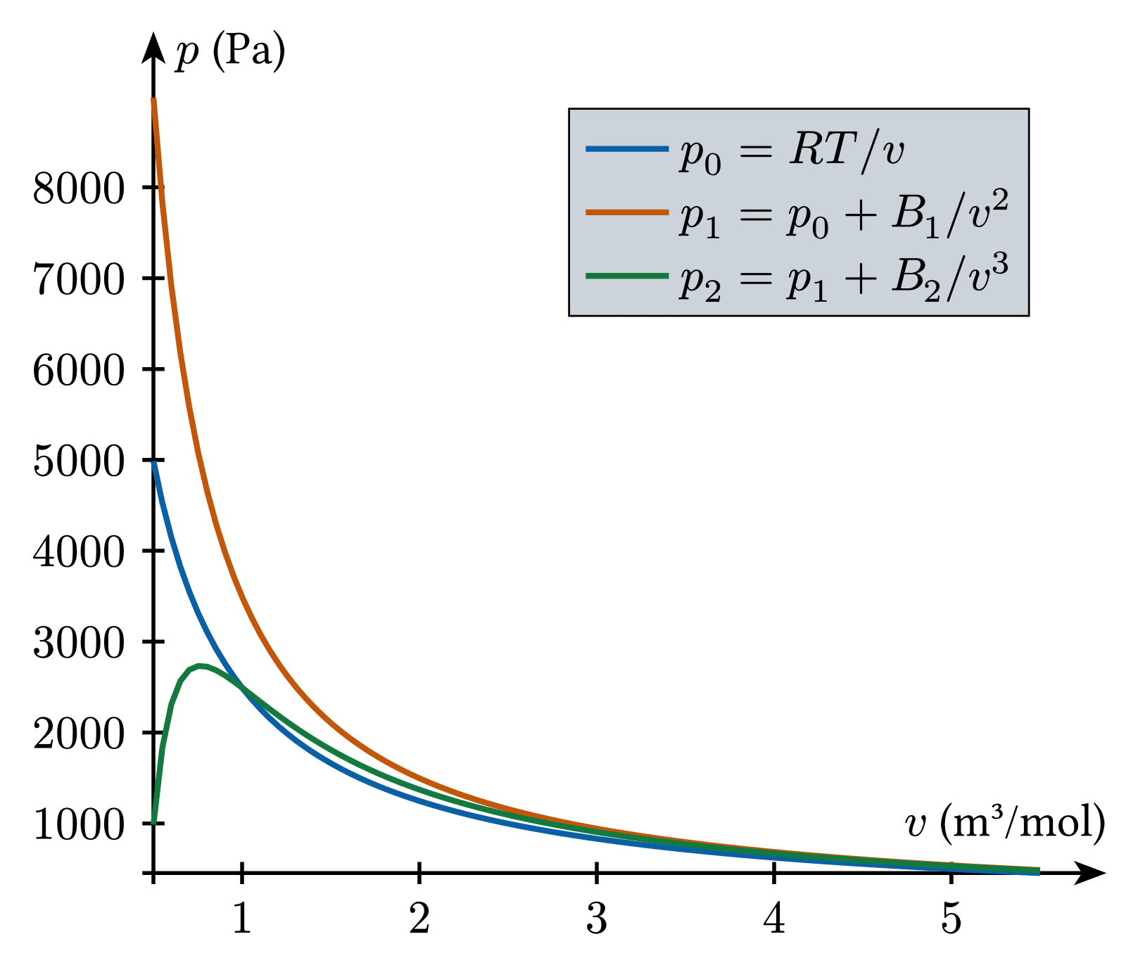
This image visualizes the behavior of gas isotherms (curves showing pressure-volume relationships at constant temperature), represented by three equations of state, as a function of volume. The equations include the ideal gas law, and its first two virial corrections $B_1 / v^2$ and $B_2 / v^3$ , which account for molecular interactions. The x-axis is the molar volume and the y-axis the pressure of the gas.

Download

PNG PDF SVG

Code

isotherms.typ (48 lines)

#import "@preview/cetz:0.5.3": canvas, draw
#import "@preview/cetz-plot:0.1.4": plot

#set page(width: auto, height: auto, margin: 8pt, fill: none)
#set text(size: 12pt)

#let gas-constant = 8.31 // J/(mol K)
#let temperature = 300 // K
#let B1 = 1000 // coefficient of the first virial correction
#let B2 = -1000 // coefficient of the second virial correction

// Ideal gas law plus successive virial corrections
#let p0(v) = gas-constant * temperature / v
#let p1(v) = p0(v) + B1 / calc.pow(v, 2)
#let p2(v) = p1(v) + B2 / calc.pow(v, 3)

#canvas({
  let axis-mark = (end: "stealth", fill: black)
  draw.set-style(axes: (
    x: (mark: axis-mark, label: (anchor: "north-east", offset: 0.6)),
    y: (mark: axis-mark, label: (anchor: "north-west", offset: -0.2)),
  ))

  plot.plot(
    size: (8, 7),
    x-label: [molar volume $v$ (m³/mol)],
    y-label: [pressure $p$ (Pa)],
    x-tick-step: 1,
    y-tick-step: 1000,
    axis-style: "left",
    legend: "inner-north-east",
    // Compact legend with a thin border.
    legend-style: (fill: rgb("#cdd3da"), item: (spacing: 0.15), padding: 0.15, stroke: 0.5pt),
    for (pressure, color, label) in (
      (p0, "#0B5FA5", [ideal gas $p_0 = R T \/ v$]),
      (p1, "#C2570A", [1st virial correction $p_1 = p_0 + B_1 \/ v^2$]),
      (p2, "#12793F", [2nd virial correction $p_2 = p_1 + B_2 \/ v^3$]),
    ) {
      plot.add(
        style: (stroke: rgb(color) + 1.5pt),
        domain: (0.5, 5.5),
        samples: 100,
        pressure,
        label: label,
      )
    },
  )
})