Ising Model Phase Transition
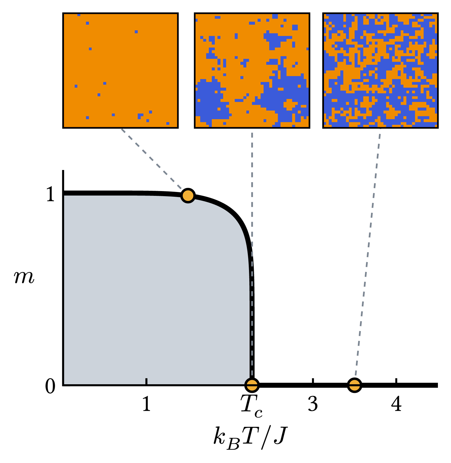
Onsager's exact spontaneous magnetization of the 2D square-lattice Ising model, , which vanishes continuously at with exponent . The snapshots come from a Metropolis Monte Carlo simulation run in Typst at , and , showing an ordered ferromagnet, large ragged domains near criticality (after 300 sweeps, still coarsening toward the fractal equilibrium clusters), and a disordered paramagnet.
Download
Code
#import "@preview/cetz:0.5.3": canvas, draw
#import draw: circle, content, line, rect

#set page(width: auto, height: auto, margin: 8pt, fill: none)
#set text(size: 15pt)

// 2D square-lattice Ising model, temperatures in units of J/k_B
#let t-c = 2 / calc.ln(1 + calc.sqrt(2)) // ≈ 2.269
#let onsager(T) = if T >= t-c { 0 } else { calc.pow(1 - calc.pow(calc.sinh(2 / T), -4), 1 / 8) }

// Metropolis Monte Carlo on an L×L periodic lattice with a MINSTD Lehmer RNG
#let L = 40
#let rng-max = 2147483647
#let next(seed) = calc.rem(seed * 48271, rng-max)
#let metropolis(T, sweeps, ordered: false, seed: 1) = {
  let s = seed
  let spins = ()
  for _ in range(L * L) {
    if ordered { spins.push(1) } else {
      s = next(s)
      spins.push(if s < rng-max / 2 { 1 } else { -1 })
    }
  }
  // acceptance thresholds for energy changes ΔE = 4J and 8J
  let accept-4 = calc.exp(-4 / T) * rng-max
  let accept-8 = calc.exp(-8 / T) * rng-max
  for _ in range(sweeps) {
    for y in range(L) {
      let row = y * L
      let up = calc.rem(y + L - 1, L) * L
      let down = calc.rem(y + 1, L) * L
      for x in range(L) {
        let i = row + x
        let neighbors = (
          spins.at(row + calc.rem(x + 1, L))
            + spins.at(row + calc.rem(x + L - 1, L))
            + spins.at(up + x)
            + spins.at(down + x)
        )
        let delta-e = 2 * spins.at(i) * neighbors
        if delta-e <= 0 { spins.at(i) = -spins.at(i) } else {
          s = next(s)
          if s < (if delta-e == 4 { accept-4 } else { accept-8 }) { spins.at(i) = -spins.at(i) }
        }
      }
    }
  }
  spins
}

#let spin-up = rgb("#f08c00")
#let spin-down = rgb("#3b5bdb")
#let rgb8(col) = col.components(alpha: false).map(v => int(calc.round(v / 100% * 255)))
#let lattice-image(spins, size) = image(
  bytes(spins.map(spin => rgb8(if spin > 0 { spin-up } else { spin-down })).join()),
  format: (encoding: "rgb8", width: L, height: L),
  width: size,
  scaling: "pixelated",
)

#let snapshots = (
  (T: 1.5, spins: metropolis(1.5, 40, ordered: true, seed: 7)),
  (T: t-c, spins: metropolis(t-c, 300, seed: 37)),
  (T: 3.5, spins: metropolis(3.5, 40, seed: 13)),
)

#canvas({
  let (width, height) = (8, 4.6)
  let (t-max, m-max) = (4.5, 1.12)
  let px(T) = T / t-max * width
  let py(m) = m / m-max * height
  let axis-stroke = 1.2pt + black
  let snap-size = 2.45
  let snap-y = height + 0.9

  // Onsager magnetization: dense sampling near T_c where m ~ (T_c − T)^(1/8)
  let n = 160
  let pts = ((0, py(1)),)
  for k in range(n + 1) {
    let T = t-c * (1 - calc.pow(1 - k / n, 6) * 0.85)
    pts.push((px(T), py(onsager(T))))
  }
  pts.push((px(t-c), 0))
  line(..pts, (0, 0), close: true, fill: rgb("#cdd3da"), stroke: none)
  line(..pts, stroke: (thickness: 3pt, join: "round"))
  line((px(t-c), 0), (px(t-max), 0), stroke: 3pt)

  // lattice snapshots linked to their temperatures on the curve
  let centers = (snap-size / 2, px(t-c), width - snap-size / 2)
  for (snap, cx) in snapshots.zip(centers) {
    let marker = (px(snap.T), py(onsager(snap.T)))
    line(marker, (cx, snap-y), stroke: (paint: rgb("#7a8591"), thickness: 1pt, dash: "dashed"))
    content((cx, snap-y), lattice-image(snap.spins, snap-size * 1cm), anchor: "south")
    rect(
      (cx - snap-size / 2, snap-y),
      (cx + snap-size / 2, snap-y + snap-size),
      stroke: 1pt + black,
    )
    circle(marker, radius: 0.14, fill: rgb("#f2b134"), stroke: 1.5pt + black)
  }

  // axes
  line((0, height), (0, 0), (width, 0), stroke: axis-stroke)
  for T in (1, 3, 4) {
    line((px(T), 0), (px(T), 0.15), stroke: axis-stroke)
    content((px(T), -0.2), str(T), anchor: "north")
  }
  content((px(t-c), -0.2), $T_c$, anchor: "north")
  for m in (0, 1) {
    line((0, py(m)), (0.15, py(m)), stroke: axis-stroke)
    content((-0.15, py(m)), str(m), anchor: "east")
  }
  content((width / 2, -0.85), $k_B T slash J$, anchor: "north")
  content((-0.6, height / 2), $m$, anchor: "east")
})