ML Activations
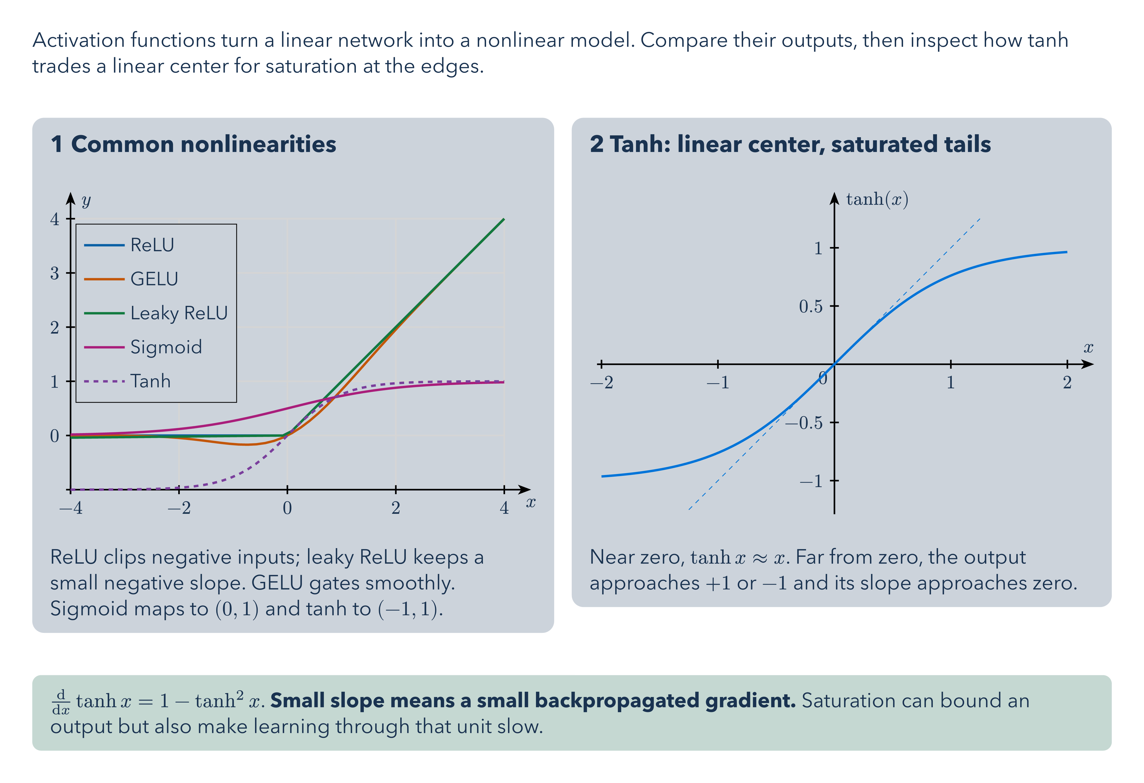
Activation functions turn a linear network into a nonlinear model. Compare their outputs, then inspect how tanh trades a linear center for saturation at the edges.
Download
Code
ml-activations.typ (157 lines)
#import "@preview/cetz:0.5.2": canvas, draw
#import "@preview/cetz-plot:0.1.4": plot
#let label-size = 12pt
#let paragraph-size = 14pt
#let heading-size = 16pt

#let card_body(title, body, caption) = block(
  width: 100%,
  inset: 12pt,
  radius: 8pt,
  fill: rgb("#cdd3da"),
  breakable: false,
)[
  #text(size: heading-size, weight: "bold", title)
  #v(8pt)
  // Measure unconstrained artwork before scaling, including content wider than its card.
  #layout(size => {
    let artwork = text(size: label-size, body)
    std.scale(size.width / measure(artwork).width * 100%, reflow: true, artwork)
  })
  #v(7pt)
  #text(size: paragraph-size, caption)
]

#let card-grid(columns: 2, ..cards) = layout(size => {
  let rows = cards
    .pos()
    .chunks(columns)
    .map(row => {
      let ratios = row.map(card => {
        let bounds = measure(text(size: label-size, card.at(1)))
        bounds.width / bounds.height
      })
      let available = size.width - 12pt * (row.len() - 1) - 24pt * row.len()
      grid(
        columns: ratios.map(ratio => 24pt + available * ratio / ratios.sum()),
        gutter: 12pt,
        ..row.map(args => card_body(..args)),
      )
    })
  stack(dir: ttb, spacing: 12pt, ..rows)
})

#let takeaway(body) = block(
  width: 100%,
  inset: 12pt,
  radius: 6pt,
  fill: rgb("#c6d8d2"),
  breakable: false,
  text(size: paragraph-size, body),
)

#set page(width: 780pt, height: auto, margin: 22pt, fill: none)
#set text(font: "Avenir Next", size: paragraph-size, fill: rgb("#19324f"))
#set par(leading: 0.55em)

// === 1  Common nonlinearities ===
#let figure-0 = [
  #let relu(x) = if x < 0 { 0 } else { x }
  #let gelu(x) = (
    0.5 * x * (1 + calc.tanh(calc.sqrt(2 / calc.pi) * (x + 0.044715 * calc.pow(x, 3))))
  )
  #let leaky-relu(x) = if x < 0 { 0.01 * x } else { x }
  #let sigmoid(x) = 1 / (1 + calc.exp(-x))
  #let tanh(x) = (calc.exp(x) - calc.exp(-x)) / (calc.exp(x) + calc.exp(-x))

  #canvas(length: 1.21cm, {
    draw.set-style(legend: (fill: rgb("#cdd3da")))
    let axis-mark = (end: "stealth", fill: black)
    draw.set-style(axes: (
      x: (mark: axis-mark),
      y: (mark: axis-mark, label: (anchor: "north-west", offset: -0.2)),
    ))
    plot.plot(
      size: (8, 5),
      y-tick-step: 1,
      x-tick-step: 2,
      legend: "inner-north-west",
      // Compact legend with a thin border.
      legend-style: (item: (spacing: 0.15), padding: 0.15, stroke: 0.5pt),
      axis-style: "left",
      x-grid: true,
      y-grid: true,
      {
        let curves = (
          ("ReLU", relu, rgb("#0B5FA5") + 1.5pt),
          ("GELU", gelu, rgb("#C2570A") + 1.5pt),
          ("Leaky ReLU", leaky-relu, rgb("#12793F") + 1.5pt),
          ("Sigmoid", sigmoid, rgb("#A81E7A") + 1.5pt),
          // Dashes distinguish the less separable purple curve.
          ("Tanh", tanh, (paint: rgb("#7A3E9D"), thickness: 1.5pt, dash: "dashed")),
        )
        for (key, func, stroke) in curves {
          plot.add(style: (stroke: stroke), domain: (-4, 4), func, label: key)
        }
      },
    )
  })
]

// === 2  Tanh: linear center, saturated tails ===
#let figure-1 = canvas(length: 1.3cm, {
  draw.set-style(legend: (fill: rgb("#cdd3da")))
  let axis-mark = (end: "stealth", fill: black)
  draw.set-style(axes: (
    x: (mark: axis-mark, label: (anchor: "south-east", offset: -0.2)),
    y: (mark: axis-mark, label: (anchor: "north-west", offset: -0.2)),
  ))

  plot.plot(
    size: (8, 5),
    x-label: $x$,
    y-label: $tanh(x)$,
    y-max: 1.25,
    y-min: -1.25,
    x-max: 2,
    x-min: -2,
    x-tick-step: 1,
    y-tick-step: 0.5,
    axis-style: "school-book",
    {
      // Main tanh curve
      plot.add(
        style: (stroke: blue + 1.5pt),
        domain: (-2, 2),
        samples: 100,
        x => calc.tanh(x),
      )

      // Dashed line y=x from -1 to 1
      plot.add(
        style: (stroke: (dash: "dashed", paint: blue, thickness: 0.5pt)),
        samples: 2,
        domain: (-1.4, 1.4),
        x => { x },
      )
    },
  )
})

Activation functions turn a linear network into a nonlinear model. Compare their outputs, then inspect how tanh trades a linear center for saturation at the edges.
#v(14pt)
#card-grid(
  (
    [1  Common nonlinearities],
    figure-0,
    [ReLU clips negative inputs; leaky ReLU keeps a small negative slope. GELU gates smoothly. Sigmoid maps to $(0,1)$ and tanh to $(-1,1)$.],
  ),
  (
    [2  Tanh: linear center, saturated tails],
    figure-1,
    [Near zero, $tanh x approx x$. Far from zero, the output approaches $+1$ or $-1$ and its slope approaches zero.],
  ),
)
#v(12pt)
#takeaway[$dif/(dif x) tanh x = 1-tanh^2 x$. *Small slope means a small backpropagated gradient.* Saturation can bound an output but also make learning through that unit slow.]