home

Maxwell Boltzmann Distribution

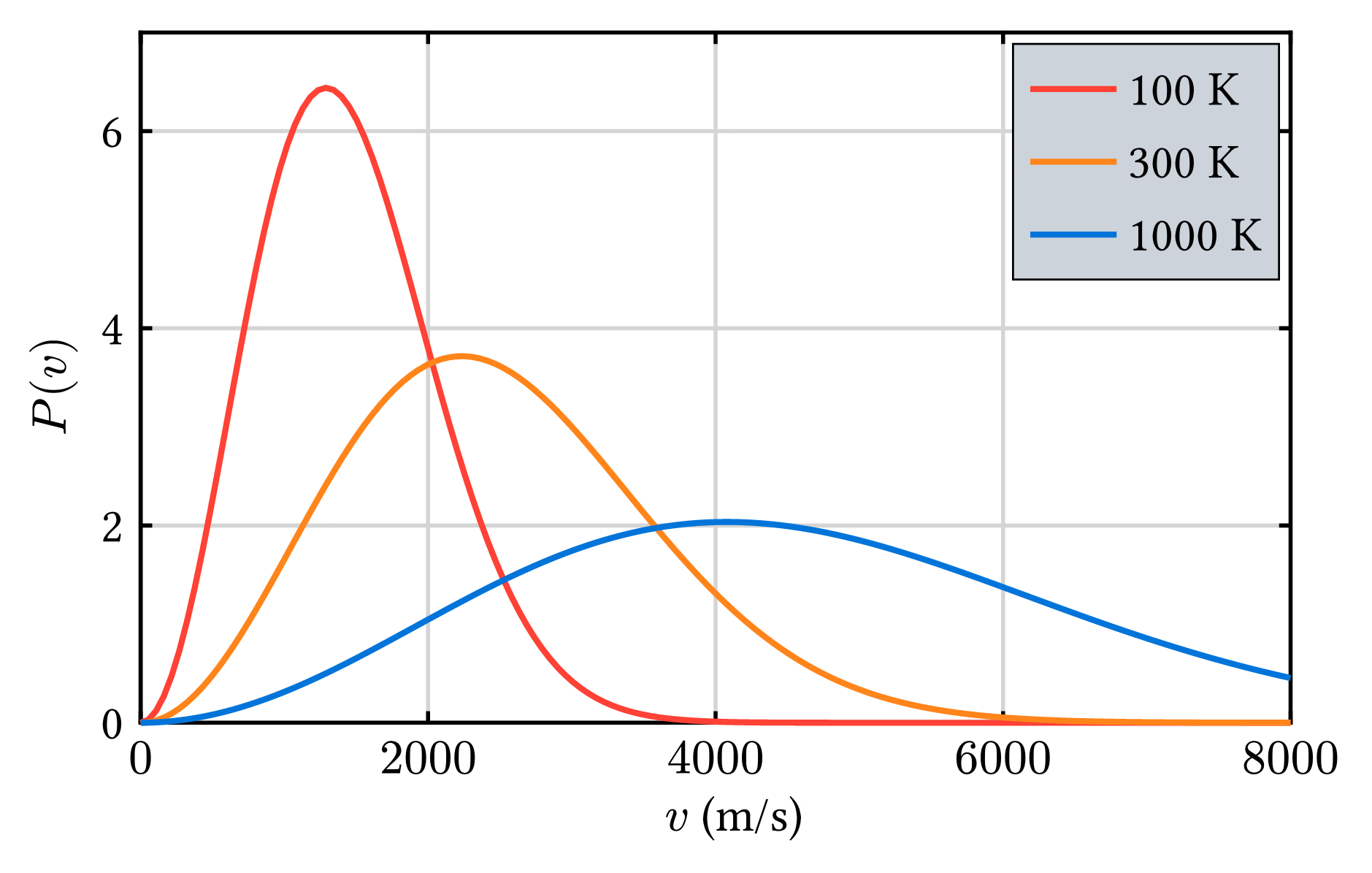
The Maxwell-Boltzmann speed distribution $P(v)$ for ideal gas particles of mass 1 u at 100, 300 and 1000 K. Higher temperatures broaden and flatten the curve, and the most probable speed $v_p = \sqrt{2 k_B T / m}$ grows with the square root of temperature.

Download

PNG PDF SVG

Code

maxwell-boltzmann-distribution.typ (41 lines)

#import "@preview/cetz:0.5.3": canvas
#import "@preview/cetz-plot:0.1.4": plot

#set page(width: auto, height: auto, margin: 8pt, fill: none)
#set text(size: 12pt)

// Constants (in SI units)
#let k-B = 1.38e-23 // Boltzmann constant
#let m-u = 1.66e-27 // unified atomic mass unit, used as the particle mass

// Maxwell-Boltzmann speed distribution
#let maxwell-boltzmann(speed, T) = {
  let prefactor = calc.pow(m-u / (2 * calc.pi * k-B * T), 3 / 2)
  4 * calc.pi * prefactor * calc.pow(speed, 2) * calc.exp(-m-u * calc.pow(speed, 2) / (2 * k-B * T))
}

#canvas({
  plot.plot(
    size: (10, 6),
    x-label: [speed $v$ (m/s)],
    y-label: [probability density $P(v)$ ($10^(-4)$ s/m)],
    y-max: 0.7e-3,
    x-tick-step: 2000,
    y-tick-step: 2e-4,
    y-format: y => calc.round(1e4 * y, digits: 2),
    legend: "inner-north-east",
    x-grid: true,
    y-grid: true,
    // Compact legend with a thin border.
    legend-style: (fill: rgb("#cdd3da"), item: (spacing: 0.15), padding: 0.15, stroke: 0.5pt),
    for (temp, color) in ((100, red), (300, orange.darken(25%)), (1000, blue)) {
      plot.add(
        style: (stroke: color + 1.5pt),
        domain: (0, 8000),
        samples: 150,
        speed => maxwell-boltzmann(speed, temp),
        label: [$T =$ #temp K],
      )
    },
  )
})