Random Phase Approximation
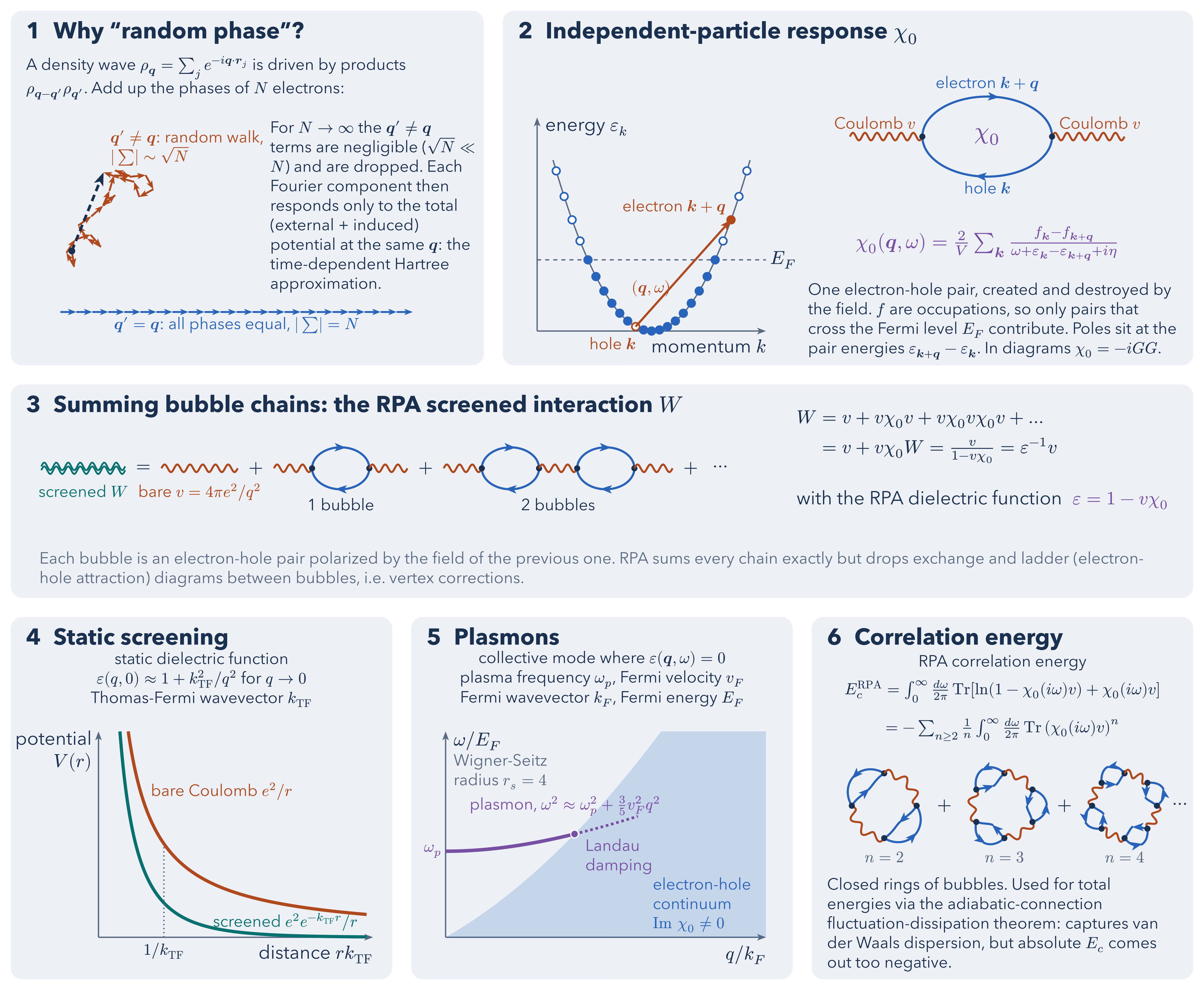
The random phase approximation (RPA) in six panels. (1) The name: a density fluctuation couples to products . For the phases of all electrons agree and add to ; for they are effectively random and their sum is a random walk of length , drawn here from 22 pseudo-random phases. Dropping those terms leaves each Fourier component responding only to the total potential at the same , the time-dependent Hartree approximation. (2) The independent-particle (Lindhard) response is one electron-hole bubble: an electron is lifted from inside the Fermi sea to an empty state , and only pairs across contribute.
(3) Summing all chains of bubbles connected by bare Coulomb lines gives the geometric series with the RPA dielectric function ; exchange and ladder diagrams between bubbles (vertex corrections) are left out. Three consequences: (4) static screening, whose long-wavelength limit turns into the Thomas-Fermi form ; (5) plasmons at the zeros of , drawn with the long-wavelength dispersion for until it enters the electron-hole continuum and is Landau damped; and (6) the RPA correlation energy, a sum of closed rings of bubbles integrated over imaginary frequencies, used for total energies through the adiabatic-connection fluctuation-dissipation theorem.
Download
Code
#import "@preview/cetz:0.5.3": canvas, draw
#import draw: circle, clip, content, line, rect

// Random phase approximation: why off-diagonal density couplings average out, the Lindhard
// bubble chi_0, the geometric series W = v / (1 - v chi_0) and three consequences. Energies in
// units of E_F and momenta in k_F (epsilon_k = k^2); the plasmon panel uses r_s = 4 (about Na).
// https://doi.org/10.1103/PhysRev.92.609 https://doi.org/10.1103/PhysRev.106.364
#set page(width: auto, height: auto, margin: 8pt, fill: none)
#let (ink, muted, panel-fill) = (rgb("#19304E"), rgb("#5A6A80"), rgb("#EDF1F6"))
#set text(font: "Avenir Next", size: 14pt, fill: ink)
#set par(leading: 0.5em)
// Fermion lines, bare Coulomb v, screened W, response chi_0
#let (c-el, c-v, c-w, c-chi) = ("#2864BB", "#B04A1C", "#06716E", "#7750A3").map(rgb)

#let small(body, ..args) = text(size: 12pt, ..args, body)
#let tip(color, scale) = (end: "stealth", fill: color, scale: scale)
#let mapper(origin, width, height, (x0, x1), (y0, y1)) = ((x, y)) => (
  origin.at(0) + (x - x0) / (x1 - x0) * width,
  origin.at(1) + (y - y0) / (y1 - y0) * height,
)
#let axes(to-canvas, (x0, x1), (y0, y1), x-label, y-label, y-axis-x: 0) = {
  line(to-canvas((x0, 0)), to-canvas((x1, 0)), stroke: muted + 1pt, mark: tip(muted, 0.7))
  line(to-canvas((y-axis-x, y0)), to-canvas((y-axis-x, y1)), stroke: muted + 1pt, mark: tip(
    muted,
    0.7,
  ))
  content(to-canvas((x1, 0)), x-label, anchor: "north-east", padding: (top: 6pt))
  content(to-canvas((y-axis-x, y1)), y-label, anchor: "north-west", padding: (left: 6pt))
}
#let samples((x0, x1), n: 200) = range(n + 1).map(idx => x0 + (x1 - x0) * idx / n)
#let panel((x0, y0), (x1, y1), title) = {
  rect((x0, y0), (x1, y1), fill: panel-fill, stroke: none, radius: 0.3)
  content((x0 + 0.4, y0 - 0.3), text(17pt, weight: "bold", title), anchor: "north-west")
}

// === Feynman parts on parametric curves p(t), t in [0, 1] ===
#let straight(start, end) = frac => start.zip(end).map(((from, to)) => from + (to - from) * frac)
#let arc((cx, cy), rx, ry, start, sweep) = frac => (
  cx + rx * calc.cos(start + sweep * frac),
  cy + ry * calc.sin(start + sweep * frac),
)
// Boson line: a sine wave about the curve, displaced by offset along its normal
#let wavy(curve, waves: 4, amp: 0.1, offset: 0, color: c-v, width: 1.5pt) = line(
  ..range(waves * 16 + 1).map(idx => {
    let frac = idx / (waves * 16)
    let ((x1, y1), (x2, y2)) = (curve(calc.max(frac - 1e-3, 0)), curve(calc.min(frac + 1e-3, 1)))
    let shift = (offset + amp * calc.sin(2 * calc.pi * waves * frac)) / calc.norm(x2 - x1, y2 - y1)
    let (x, y) = curve(frac)
    (x - (y2 - y1) * shift, y + (x2 - x1) * shift)
  }),
  stroke: color + width,
)
#let n-waves(start, end) = calc.max(2, int(calc.round(
  calc.norm(..start.zip(end).map(((from, to)) => to - from)) / 0.32,
)))
#let coulomb(start, end) = wavy(straight(start, end), waves: n-waves(start, end))
#let screened(start, end) = for offset in (-0.05, 0.05) {
  wavy(straight(start, end), waves: n-waves(start, end), offset: offset, color: c-w, width: 1.3pt)
}
// Fermion propagator with a direction arrow at its midpoint
#let fermion(curve, color: c-el, width: 1.6pt) = {
  let pts(from, to) = range(31).map(idx => curve(from + (to - from) * idx / 30))
  line(..pts(0, 0.56), stroke: color + width, mark: tip(color, 0.75))
  line(..pts(0.5, 1), stroke: color + width)
}
#let vertex(pos) = circle(pos, radius: 0.08, fill: ink, stroke: none)
// Electron-hole bubble between (cx - rx, y) and (cx + rx, y): particle on top, hole below
#let bubble((cx, y), rx, ry) = {
  fermion(arc((cx, y), rx, ry, 180deg, -180deg))
  fermion(arc((cx, y), rx, ry, 0deg, -180deg))
  for x in (cx - rx, cx + rx) { vertex((x, y)) }
}
// v chi_0 v chi_0 ... v with n bubbles, starting at x0 and chain-len(n) long
#let (chain-leg, chain-bubble) = (1, 1.5)
#let chain-len(n, leg: chain-leg, bw: chain-bubble) = (n + 1) * leg + n * bw
#let chain(x0, y, n, leg: chain-leg, bw: chain-bubble, ry: 0.55) = for idx in range(n + 1) {
  let x = x0 + idx * (leg + bw)
  coulomb((x, y), (x + leg, y))
  if idx < n { bubble((x + leg + bw / 2, y), bw / 2, ry) }
}

// === Panel 1: phases of N electrons ===
#let n-el = 22
#let step = 0.42
#let noise(idx) = calc.rem-euclid(calc.sin(idx * 12.9898 + 78.233) * 43758.5453, 1)
#let phases = range(n-el).map(idx => 2 * calc.pi * noise(idx))
#let resultant = (phases.map(calc.cos).sum(), phases.map(calc.sin).sum())
// A global phase is arbitrary: rotate the walk so its resultant points up and to the right
#let rotation = 68deg - calc.atan2(..resultant)
#let walk = phases.fold(((0, 0),), (acc, phi) => {
  let (x, y) = acc.last()
  acc + ((x + step * calc.cos(phi * 1rad + rotation), y + step * calc.sin(phi * 1rad + rotation)),)
})

// === Panel 5: free-electron gas at r_s = 4, units E_F and k_F ===
#let r-s = 4
#let k-fermi = calc.pow(9 * calc.pi / 4, 1 / 3) / r-s
#let omega-p = calc.sqrt(3 / calc.pow(r-s, 3)) / (k-fermi * k-fermi / 2)
// Long-wavelength RPA dispersion; v_F = 2 in these units
#let plasmon(q) = calc.sqrt(omega-p * omega-p + 3 / 5 * 4 * q * q)
#let (eh-max, eh-min) = (q => q * q + 2 * q, q => calc.max(0, q * q - 2 * q))
#let q-damp = samples((0, 2), n: 4000).find(q => plasmon(q) <= eh-max(q))
#assert(1.8 < omega-p and omega-p < 1.95 and 0.75 < q-damp and q-damp < 0.85, message: repr((
  omega-p,
  q-damp,
)))

#canvas(length: 1cm, {
  // === 1: random phases ===
  panel((0, 0), (12.4, -9.3), [1 #h(0.3em) Why "random phase"?])
  let intro = [A density wave $rho_bold(q) = sum_j e^(-i bold(q) dot bold(r)_j)$ is driven by products $rho_(bold(q) - bold(q)') rho_(bold(q)')$. Add up the phases of $N$ electrons:]
  content((0.4, -1.25), box(width: 11.6cm, small(intro)), anchor: "north-west")
  let origin = (1.3, -7.9)
  let on-row((x, y)) = (origin.at(0) + x, origin.at(1) + y)
  for idx in range(n-el) {
    let x = idx * step
    line(on-row((x, 0)), on-row((x + step, 0)), stroke: c-el + 1.4pt, mark: tip(c-el, 0.45))
  }
  content(
    on-row((n-el * step / 2, -0.15)),
    small(fill: c-el)[$bold(q)' = bold(q)$: all phases equal, $|sum| = N$],
    anchor: "north",
  )
  let on-walk((x, y)) = (1.6 + x, -6.3 + y)
  for (from, to) in walk.zip(walk.slice(1)) {
    line(on-walk(from), on-walk(to), stroke: c-v + 1.4pt, mark: tip(c-v, 0.45))
  }
  line(
    on-walk((0, 0)),
    on-walk(walk.last()),
    stroke: (paint: ink, thickness: 2pt, dash: (5pt, 3pt)),
    mark: tip(ink, 0.8),
  )
  circle(on-walk((0, 0)), radius: 0.09, fill: ink, stroke: none)
  let random-label = [$bold(q)' != bold(q)$: random walk,\ $|sum| tilde sqrt(N)$]
  content(on-walk(walk.last()), small(fill: c-v, random-label), anchor: "south-west", padding: 5pt)
  let keep = [For $N -> oo$ the $bold(q)' != bold(q)$ terms are negligible ($sqrt(N) << N$) and are dropped. Each Fourier component then responds only to the total (external + induced) potential at the same $bold(q)$: the time-dependent Hartree approximation.]
  content((6.8, -2.9), box(width: 5.4cm, small(keep)), anchor: "north-west")

  // === 2: Lindhard bubble ===
  panel((12.9, 0), (31, -9.3), [2 #h(0.3em) Independent-particle response $chi_0$])
  let (k-lim, e-lim) = ((-1.8, 1.8), (0, 3))
  let to-canvas = mapper((13.8, -8.4), 6, 5.6, k-lim, e-lim)
  axes(to-canvas, k-lim, e-lim, [momentum $k$], [energy $epsilon_k$], y-axis-x: -1.8)
  line(..samples((-1.55, 1.55)).map(k => to-canvas((k, k * k))), stroke: muted + 1pt)
  line(to-canvas((-1.8, 1)), to-canvas((1.8, 1)), stroke: (
    paint: muted,
    thickness: 1pt,
    dash: "dashed",
  ))
  content(to-canvas((1.8, 1)), $E_F$, anchor: "west", padding: 3pt)
  let (k-hole, k-elec) = (-0.25, 1.25)
  for idx in range(25) {
    let k = -1.5 + idx / 8
    let filled = calc.abs(k) <= 1 and k != k-hole or k == k-elec
    let color = if k in (k-hole, k-elec) { c-v } else { c-el }
    circle(
      to-canvas((k, k * k)),
      radius: 0.1,
      fill: if filled { color } else { white },
      stroke: color + 1.2pt,
    )
  }
  line(
    to-canvas((k-hole, k-hole * k-hole)),
    to-canvas((k-elec, k-elec * k-elec)),
    stroke: c-v + 1.6pt,
    mark: tip(c-v, 0.7),
  )
  content(to-canvas((0.3, 0.6)), small(fill: c-v)[$(bold(q), omega)$], anchor: "east")
  content(to-canvas((k-hole, 0)), small(fill: c-v)[hole $bold(k)$], anchor: "north-east", padding: (
    top: 5pt,
  ))
  content(
    to-canvas((k-elec, k-elec * k-elec)),
    small(fill: c-v)[electron $bold(k) + bold(q)$],
    anchor: "south-east",
    padding: 4pt,
  )
  let (cx, cy) = (25.6, -3.3)
  coulomb((cx - 3.6, cy), (cx - 1.7, cy))
  coulomb((cx + 1.7, cy), (cx + 3.6, cy))
  bubble((cx, cy), 1.7, 1.05)
  content((cx, cy), text(fill: c-chi, 18pt)[$chi_0$])
  content(
    (cx, cy + 1.05),
    small(fill: c-el)[electron $bold(k) + bold(q)$],
    anchor: "south",
    padding: 4pt,
  )
  content((cx, cy - 1.05), small(fill: c-el)[hole $bold(k)$], anchor: "north", padding: 4pt)
  content((cx - 2.95, cy + 0.2), small(fill: c-v)[Coulomb $v$], anchor: "south")
  content((cx + 2.95, cy + 0.2), small(fill: c-v)[Coulomb $v$], anchor: "south")
  let lindhard = $chi_0(bold(q), omega) = 2 / V sum_bold(k) (f_bold(k) - f_(bold(k) + bold(q))) / (omega + epsilon_bold(k) - epsilon_(bold(k) + bold(q)) + i eta)$
  content((cx, -6.1), text(fill: c-chi, 15pt, lindhard))
  let pauli = [One electron-hole pair, created and destroyed by the field. $f$ are occupations, so only pairs that cross the Fermi level $E_F$ contribute. Poles sit at the pair energies $epsilon_(bold(k) + bold(q)) - epsilon_bold(k)$. In diagrams $chi_0 = -i G G$.]
  content((20.9, -7.15), box(width: 9.7cm, small(pauli)), anchor: "north-west")

  // === 3: geometric series ===
  panel(
    (0, -9.8),
    (31, -15.4),
    [3 #h(0.3em) Summing bubble chains: the RPA screened interaction $W$],
  )
  let y = -12
  let (x, gap) = (0.8, 0.95)
  screened((x, y), (x + 2.2, y))
  content((x + 1.1, y - 0.45), small(fill: c-w)[screened $W$], anchor: "north")
  x += 2.2
  content((x + gap / 2, y), $=$)
  x += gap
  coulomb((x, y), (x + 2, y))
  content((x + 1, y - 0.45), small(fill: c-v)[bare $v = 4 pi e^2 slash q^2$], anchor: "north")
  x += 2
  for n in (1, 2) {
    content((x + gap / 2, y), $+$)
    x += gap
    chain(x, y, n)
    let len = chain-len(n)
    content((x + len / 2, y - 0.8), small[#n bubble#if n > 1 [s]], anchor: "north")
    x += len
  }
  content((x + gap / 2, y), $+$)
  content((x + gap + 0.3, y), $dots.c$)
  let algebra = [
    $W & = v + v chi_0 v + v chi_0 v chi_0 v + dots \
    & = v + v chi_0 W = v / (1 - v chi_0) = epsilon^(-1) v$
    #v(4pt)
    with the RPA dielectric function #h(0.3em) #text(fill: c-chi)[$epsilon = 1 - v chi_0$]
  ]
  content((20.6, -11.95), algebra, anchor: "west")
  let series-note = [Each bubble is an electron-hole pair polarized by the field of the previous one. RPA sums every chain exactly but drops exchange and ladder (electron-hole attraction) diagrams between bubbles, i.e. vertex corrections.]
  content((15.5, -14.2), box(width: 29.5cm, small(fill: muted, series-note)), anchor: "north")

  // === 4: static screening ===
  panel((0, -15.9), (10, -25.4), [4 #h(0.3em) Static screening])
  content((5, -17.55), small(align(
    center,
  )[static dielectric function \ $epsilon(q, 0) approx 1 + k_"TF"^2 slash q^2$ for $q -> 0$ \ Thomas-Fermi wavevector $k_"TF"$]))
  let (r-lim, v-lim) = ((0, 4.2), (0, 2.2))
  let to-canvas = mapper((2.3, -24.3), 7.2, 5.4, r-lim, v-lim)
  axes(to-canvas, r-lim, v-lim, [distance $r k_"TF"$], [])
  content(to-canvas((0, 2.2)), align(right)[potential\ $V(r)$], anchor: "north-east", padding: (
    right: 5pt,
  ))
  clip(rect(to-canvas((0, 0)), to-canvas((4.2, 2.2))), {
    line(..samples((0.3, 4.1)).map(r => to-canvas((r, 1 / r))), stroke: c-v + 2.4pt)
    line(..samples((0.05, 4.1)).map(r => to-canvas((r, calc.exp(-r) / r))), stroke: c-w + 2.4pt)
  })
  line(to-canvas((1, 0)), to-canvas((1, 1)), stroke: (paint: muted, thickness: 1pt, dash: "dotted"))
  content(to-canvas((1, 0)), small[$1 slash k_"TF"$], anchor: "north", padding: (top: 4pt))
  content(to-canvas((0.8, 1.55)), small(fill: c-v)[bare Coulomb $e^2 slash r$], anchor: "west")
  content(
    to-canvas((1.75, 0.07)),
    small(fill: c-w)[screened $e^2 e^(-k_"TF" r) slash r$],
    anchor: "south-west",
  )

  // === 5: plasmons ===
  panel((10.5, -15.9), (20.5, -25.4), [5 #h(0.3em) Plasmons])
  content((15.5, -17.55), small(align(
    center,
  )[collective mode where $epsilon(bold(q), omega) = 0$ \ plasma frequency $omega_p$, Fermi velocity $v_F$ \ Fermi wavevector $k_F$, Fermi energy $E_F$]))
  let (q-lim, w-lim) = ((0, 2), (0, 4.5))
  let to-canvas = mapper((11.4, -24.3), 8.4, 5.4, q-lim, w-lim)
  axes(to-canvas, q-lim, w-lim, $q slash k_F$, $omega slash E_F$)
  let qs = samples((0, 2))
  line(
    ..qs.map(q => to-canvas((q, calc.min(eh-max(q), 4.5)))),
    ..qs.rev().map(q => to-canvas((q, eh-min(q)))),
    close: true,
    fill: c-el.transparentize(80%),
    stroke: none,
  )
  clip(rect(to-canvas((0, 0)), to-canvas((2, 4.5))), {
    line(..samples((0, q-damp)).map(q => to-canvas((q, plasmon(q)))), stroke: c-chi + 2.6pt)
    line(..samples((q-damp, 1.2)).map(q => to-canvas((q, plasmon(q)))), stroke: (
      paint: c-chi,
      thickness: 2pt,
      dash: "dotted",
    ))
  })
  circle(to-canvas((q-damp, plasmon(q-damp))), radius: 0.1, fill: c-chi, stroke: white + 0.8pt)
  content(to-canvas((0, omega-p)), small(fill: c-chi)[$omega_p$], anchor: "east", padding: 3pt)
  content(
    to-canvas((0.15, 2.85)),
    small(fill: c-chi)[plasmon, $omega^2 approx omega_p^2 + 3/5 v_F^2 q^2$],
    anchor: "west",
  )
  content(
    to-canvas((0.05, 4)),
    small(fill: muted)[Wigner-Seitz\ radius $r_s = #r-s$],
    anchor: "north-west",
  )
  content(
    to-canvas((q-damp, plasmon(q-damp))),
    small(fill: c-chi)[Landau\ damping],
    anchor: "north-west",
    padding: (left: 8pt, top: 4pt),
  )
  content(to-canvas((1.6, 0.7)), small(fill: c-el)[electron-hole\ continuum\ $"Im" chi_0 != 0$])

  // === 6: ring diagrams ===
  panel((21, -15.9), (31, -25.4), [6 #h(0.3em) Correlation energy])
  let e-c = [$E_c^"RPA" = integral_0^oo (d omega) / (2 pi) op("Tr")[ln(1 - chi_0(i omega) v) + chi_0(i omega) v]$]
  content((26, -17.1), small[RPA correlation energy])
  content((26, -17.85), small(e-c))
  content(
    (26, -18.85),
    small[$= -sum_(n >= 2) 1 / n integral_0^oo (d omega) / (2 pi) op("Tr")(chi_0(i omega) v)^n$],
  )
  let ring((cx, cy), n, radius: 0.85, h: 0.26) = {
    let unit = 360deg / n
    let beta = unit * 0.5
    for idx in range(n) {
      let th0 = 90deg + idx * unit
      let polar(r, th) = (cx + r * calc.cos(th), cy + r * calc.sin(th))
      fermion(frac => polar(radius + h * calc.sin(180deg * frac), th0 + beta * frac))
      fermion(frac => polar(radius - h * calc.sin(180deg * frac), th0 + beta * (1 - frac)))
      wavy(arc((cx, cy), radius, radius, th0 + beta, unit - beta), waves: calc.max(2, int(
        calc.round(4 / n + 0.5),
      )))
      for th in (th0, th0 + beta) { vertex(polar(radius, th)) }
    }
  }
  for (idx, n) in (2, 3, 4).enumerate() {
    let cx = 22.9 + idx * 3.15
    ring((cx, -20.85), n)
    content((cx, -22.05), small(fill: muted)[$n = #n$], anchor: "north")
    if idx > 0 { content((cx - 1.575, -20.85), $+$) }
  }
  content((30.65, -20.85), $dots.c$)
  let ring-note = [Closed rings of bubbles. Used for total energies via the adiabatic-connection fluctuation-dissipation theorem: captures van der Waals dispersion, but absolute $E_c$ comes out too negative.]
  content((21.4, -22.75), box(width: 9.2cm, small(ring-note)), anchor: "north-west")
})