Wannierization and Wannier Centers
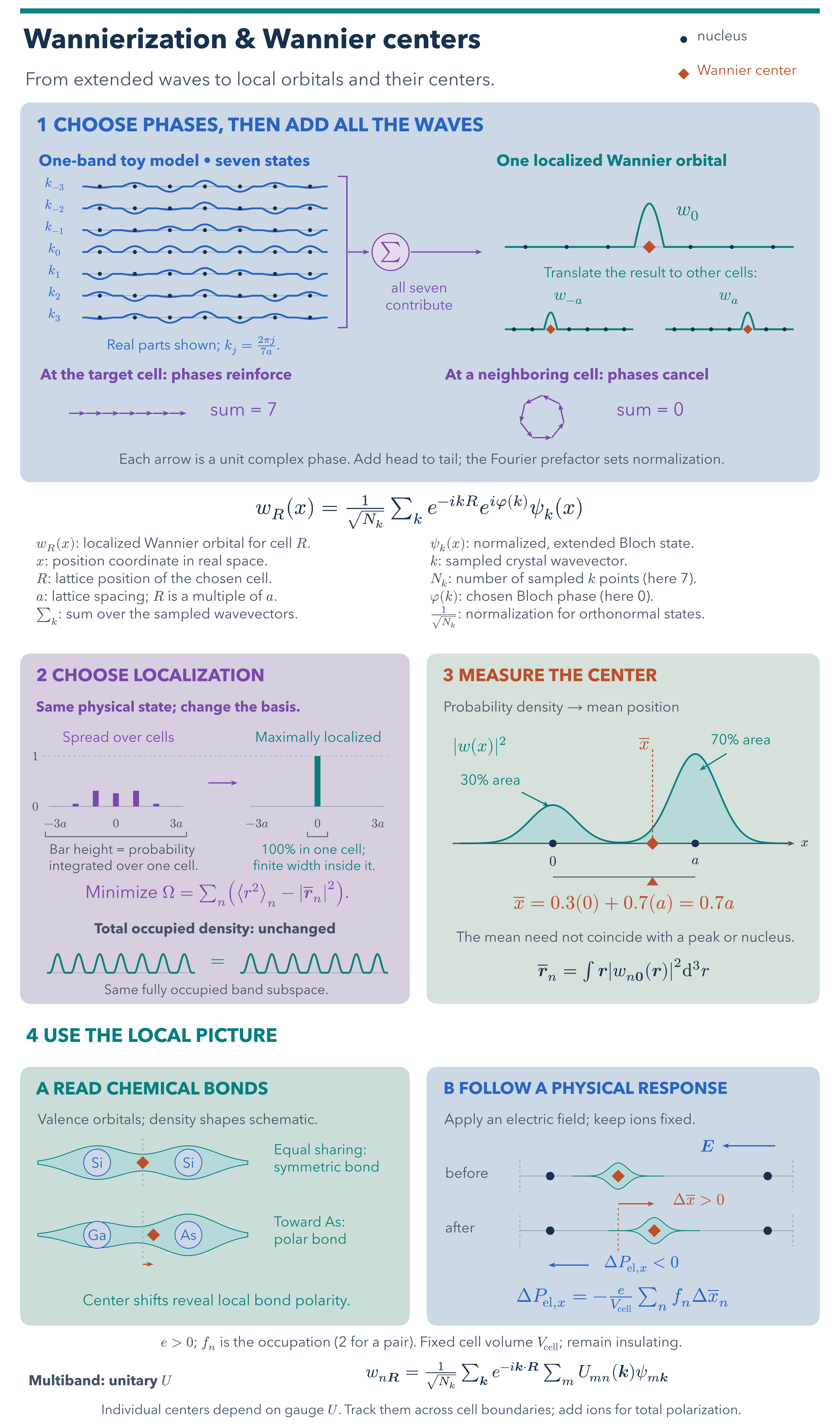
One combined diagram explains phase alignment, Fourier synthesis, localization, and Wannier centers. Seven Bloch states feed one orbital, with phase arrows showing reinforcement and cancellation. A gauge comparison preserves the total occupied density, while a 30/70 Gaussian mixture and balance diagram place the mean at 0.7a. Applications contrast symmetric Si–Si and polar Ga–As bonding, then illustrate an insulator's polarization response to an electric field.
The one-band toy model uses seven disjoint normalized cosine orbitals and orthonormal Bloch states in a periodic supercell. Exact single-cell confinement is specific to this model; the brackets show cell ranges, not RMS widths. Gauge probabilities use exp(i 1.5 cos(ka)) and constant phases. Bond clouds are schematic Gaussian mixtures. Individual centers depend on gauge. Polarization changes assume fixed occupations and cell volume along a continuous insulating path; follow centers across cell boundaries and add ionic contributions for total polarization. Entangled bands first require a suitable subspace, and the selected bands must admit localized Wannier functions.
Download
Code
wannierization-and-wannier-centers.typ (497 lines)
#import "@preview/cetz:0.5.2": canvas, draw
#import draw: circle, content, line, rect

// Bloch/Wannier conventions: orthonormal Bloch states on a finite periodic mesh.
// The toy band uses seven disjoint, normalized cosine orbitals, one per cell.
// Their discrete Fourier transform is exact. Panel 1 shows all seven real parts
// and head-to-tail unit phase vectors at cell 0 and neighboring cell 1.
// Gauge comparison: U(k) = exp(i * strength * cos(ka)), evaluated on the same mesh.
// The bond density is a separate normalized Gaussian-mixture illustration.
// Bond examples: valence MLWFs in Si and GaAs; the GaAs center is 0.617 of the
// bond length from Ga in Marzari & Vanderbilt, Phys. Rev. B 56, 12847 (1997).
// Polarization: fixed cell, fixed occupations, and continuously tracked centers
// along an insulating path. The sketch isolates the electronic contribution.
// References: Marzari et al., Rev. Mod. Phys. 84, 1419 (2012), sections II, IV, V.
// https://doi.org/10.1103/RevModPhys.84.1419
// https://doi.org/10.1103/PhysRevB.56.12847
// https://wannier90.readthedocs.io/en/latest/tutorials/tutorial_9/
// https://wannier90.readthedocs.io/en/latest/user_guide/wannier90/methodology/
#set page(width: auto, height: auto, margin: 0pt, fill: none)
#set text(font: "Avenir Next", size: 18pt, fill: rgb("#19304E"))
#set par(leading: 0.5em)
#set math.equation(numbering: none)

#let ink = rgb("#19304E")
#let muted = rgb("#43536A")
#let blue = rgb("#2764C3")
#let teal = rgb("#087F7C")
#let orange = rgb("#BC502D")
#let purple = rgb("#7948AD")
#let grid_color = rgb("#98A7B8")
#let cell_indices = range(-3, 4)
#let cell_count = cell_indices.len()
#let orbital_halfwidth = 0.36

// Compact support makes neighboring orbitals orthogonal without an overlap model.
#let local_orbital(position) = if calc.abs(position) < orbital_halfwidth {
  calc.cos(calc.pi * position / (2 * orbital_halfwidth)) / calc.sqrt(orbital_halfwidth)
} else { 0 }
#let bloch_real(position, wave_idx) = {
  // Compact support leaves only the nearest cell's orbital in the Bloch sum.
  let cell_idx = int(calc.round(position))
  if not cell_indices.contains(cell_idx) { return 0 }
  let phase = 2 * calc.pi * wave_idx * cell_idx / cell_count
  calc.cos(phase) * local_orbital(position - cell_idx) / calc.sqrt(cell_count)
}
#let phase_angle(wave_idx, cell_idx, strength: 0) = {
  let wave_phase = 2 * calc.pi * wave_idx / cell_count
  wave_phase * cell_idx + strength * calc.cos(wave_phase)
}
#let make_gauge(strength) = {
  // Compute every site–orbital displacement once; retain the original sum order.
  let min_offset = cell_indices.first() - cell_indices.last()
  let weights = range(min_offset, 1 - min_offset).map(cell_idx => {
    let phases = cell_indices.map(wave_idx => phase_angle(wave_idx, cell_idx, strength: strength))
    let real_part = phases.map(calc.cos).sum() / cell_count
    let imag_part = phases.map(calc.sin).sum() / cell_count
    real_part * real_part + imag_part * imag_part
  })
  (
    probabilities: cell_indices.map(cell_idx => weights.at(cell_idx - min_offset)),
    density: position => {
      // Disjoint support leaves only the nearest site's contribution.
      let site_cell = int(calc.round(position))
      if not cell_indices.contains(site_cell) { return 0 }
      let site_density = calc.pow(local_orbital(position - site_cell), 2)
      cell_indices
        .map(orbital_cell => weights.at(site_cell - orbital_cell - min_offset) * site_density)
        .sum()
    },
  )
}
#let spread_gauge = make_gauge(1.5)
#let localized_gauge = make_gauge(0)

#let gaussian(position, center, sigma) = (
  calc.exp(-0.5 * calc.pow((position - center) / sigma, 2)) / (sigma * calc.sqrt(2 * calc.pi))
)
#let make_bond(left_weight, sigma) = (
  left_weight: left_weight,
  sigma: sigma,
  center: 1 - left_weight,
  density: position => (
    left_weight * gaussian(position, 0, sigma) + (1 - left_weight) * gaussian(position, 1, sigma)
  ),
)
#let center_example = make_bond(0.3, 0.16)
#let si_bond = make_bond(0.5, 0.3)
#let gaas_bond = make_bond(1 - 0.617, 0.3)

#let label(left, top, width, body, size: 17pt, color: muted, weight: "regular", centered: false) = {
  content(
    (left, -top),
    block(width: width * 1pt)[
      #text(size: size, fill: color, weight: weight, if centered { align(center, body) } else {
        body
      })
    ],
    anchor: "north-west",
    padding: 0pt,
  )
}
#let heading = label.with(size: 21pt, weight: "bold")
#let equation = label.with(size: 22pt, color: ink, centered: true)
#let symbol(center_x, center_y, body, size: 20pt, color: ink) = {
  content(
    (center_x, -center_y),
    text(size: size, fill: color, top-edge: "bounds", bottom-edge: "bounds", body),
    anchor: "center",
    padding: 0pt,
  )
}
#let panel(left, top, width, height, fill) = {
  rect((left, -top), (left + width, -top - height), radius: 12, fill: fill, stroke: none)
}
#let guide_line(start, end, color: grid_color, thickness: 1pt) = {
  line(start, end, stroke: (paint: color, thickness: thickness, dash: "dashed"))
}
#let arrow(start_x, start_y, end_x, end_y, color: ink) = {
  line((start_x, -start_y), (end_x, -end_y), stroke: 1.5pt + color, mark: (
    start: none,
    end: "stealth",
    scale: 0.7,
    fill: color,
  ))
}
#let center_mark(center_x, center_y, radius: 6) = {
  line(
    (center_x, -center_y + radius),
    (center_x + radius, -center_y),
    (center_x, -center_y - radius),
    (center_x - radius, -center_y),
    close: true,
    fill: orange,
    stroke: 1pt + orange,
  )
}
#let wave_plot(left, baseline, width, amplitude, wave, accent, atoms: true) = {
  line((left, -baseline), (left + width, -baseline), stroke: 0.8pt + grid_color)
  let points = range(561).map(sample_idx => {
    let position = -3.5 + sample_idx / 80
    (left + (position + 3.5) * width / 7, -baseline + amplitude * wave(position))
  })
  line(..points, stroke: 2.2pt + accent)
  if atoms {
    for cell_idx in cell_indices {
      circle((left + (cell_idx + 3.5) * width / 7, -baseline), radius: 2.4, fill: ink, stroke: none)
    }
  }
}

// Unit phase arrows, placed head to tail. The sum closes for any nonzero cell
// modulo seven, and has length seven at cell zero.
#let phase_vertices(cell_idx) = {
  let vertices = ((0, 0),)
  for wave_idx in range(cell_count) {
    let phase = phase_angle(wave_idx, cell_idx)
    let (previous_x, previous_y) = vertices.last()
    vertices.push((previous_x + calc.cos(phase), previous_y + calc.sin(phase)))
  }
  vertices
}
#let phase_chain(left, baseline, cell_idx, scale) = {
  for ((start_x, start_y), (end_x, end_y)) in phase_vertices(cell_idx).windows(2) {
    arrow(
      left + scale * start_x,
      baseline - scale * start_y,
      left + scale * end_x,
      baseline - scale * end_y,
      color: purple,
    )
  }
}
#let density_cloud(left, baseline, width, amplitude, density) = {
  let samples = range(121).map(sample_idx => {
    let position = -0.65 + 2.3 * sample_idx / 120
    (
      left + (position + 0.65) * width / 2.3,
      amplitude * density(position),
    )
  })
  let upper = samples.map(((center_x, height)) => (center_x, -baseline + height))
  let lower = samples.rev().map(((center_x, height)) => (center_x, -baseline - height))
  line(..upper, ..lower, close: true, fill: teal.lighten(70%), stroke: 1pt + teal)
}

#canvas(length: 1pt, {
  rect((0, 0), (1000, -1700), fill: none, stroke: none)
  rect((24, -10), (976, -16), fill: teal, stroke: none)
  heading(28, 34, 790, size: 33pt, color: ink)[Wannierization & Wannier centers]
  label(30, 86, 770, size: 22pt)[From extended waves to local orbitals and their centers.]
  circle((814, -47), radius: 4, fill: ink, stroke: none)
  label(830, 36, 146)[nucleus]
  center_mark(814, 88)
  label(830, 77, 146, color: orange)[Wannier center]

  // === 1. Many Bloch states form each Wannier orbital ===
  panel(24, 122, 952, 452, rgb("#CCD8E5"))
  heading(43, 140, 914, size: 23pt, color: blue)[1  CHOOSE PHASES, THEN ADD ALL THE WAVES]
  heading(46, 184, 348, size: 19pt, color: blue)[One-band toy model • seven states]
  heading(591, 184, 362, size: 19pt, color: teal)[One localized Wannier orbital]
  for (row_idx, wave_idx) in cell_indices.enumerate() {
    let baseline = 222 + 26 * row_idx
    wave_plot(98, baseline, 292, 11, position => bloch_real(position, wave_idx), blue)
    symbol(65, baseline - 3, $k_#wave_idx$, size: 16pt, color: blue)
  }
  // One bracket encloses the entire basis; it cannot imply a row-by-row conversion.
  line((402, -210), (413, -210), (413, -390), (402, -390), stroke: 1.6pt + purple)
  arrow(414, 300, 440, 300, color: purple)
  circle((465, -300), radius: 22, fill: purple.lighten(80%), stroke: 1.3pt + purple)
  symbol(465, 300, $sum$, size: 24pt, color: purple)
  arrow(489, 300, 574, 300, color: purple)
  label(426, 336, 146, color: purple, centered: true)[all seven\ contribute]
  label(55, 404, 347, color: blue, centered: true)[Real parts shown; $k_j = (2pi j)/(7a)$.]

  wave_plot(601, 294, 344, 31, local_orbital, teal)
  center_mark(773, 294, radius: 7)
  symbol(819, 254, $w_0$, size: 24pt, color: teal)
  label(604, 318, 340, color: teal, centered: true)[Translate the result to other cells:]
  for (plot_left, selected_cell, orbital_label) in ((601, -1, $w_(-a)$), (792, 1, $w_a$)) {
    wave_plot(
      plot_left,
      392,
      153,
      12,
      position => local_orbital(position - selected_cell),
      teal,
    )
    center_mark(plot_left + (selected_cell + 3.5) * 153 / 7, 392, radius: 5)
    symbol(plot_left + 76, 355, orbital_label, size: 20pt, color: teal)
  }

  heading(48, 439, 422, size: 18pt, color: purple)[At the target cell: phases reinforce]
  heading(530, 439, 420, size: 18pt, color: purple)[At a neighboring cell: phases cancel]
  phase_chain(82, 492, 0, 20)
  label(250, 479, 198, size: 22pt, color: purple)[sum = 7]
  phase_chain(634, 521, 1, 23)
  label(734, 479, 201, size: 22pt, color: purple)[sum = 0]
  label(
    43,
    540,
    915,
    centered: true,
  )[Each arrow is a unit complex phase. Add head to tail; the Fourier prefactor sets normalization.]

  equation(
    34,
    594,
    931,
    size: 26pt,
  )[$w_(R)(x) = 1 / sqrt(N_k) sum_k e^(-i k R) e^(i phi(k)) psi_(k)(x)$]
  label(43, 640, 914)[
    #grid(
      columns: (1fr, 1fr),
      column-gutter: 24pt,
      row-gutter: 9pt,
      [$w_(R)(x)$: localized Wannier orbital for cell $R$.],
      [$psi_(k)(x)$: normalized, extended Bloch state.],

      [$x$: position coordinate in real space.], [$k$: sampled crystal wavevector.],
      [$R$: lattice position of the chosen cell.], [$N_k$: number of sampled $k$ points (here 7).],
      [$a$: lattice spacing; $R$ is a multiple of $a$.], [$phi(k)$: chosen Bloch phase (here 0).],
      [$sum_k$: sum over the sampled wavevectors.],
      [$1/sqrt(N_k)$: normalization for orthonormal states.],
    )
  ]

  // Leave room for the equation key without changing the lower panels' geometry.
  draw.translate((0, -100))
  // === 2. Different representations of the same occupied subspace ===
  panel(24, 678, 464, 417, rgb("#D7CFDF"))
  panel(508, 678, 468, 417, rgb("#D6E1DB"))
  heading(43, 696, 427, color: purple)[2  CHOOSE LOCALIZATION]
  heading(43, 735, 427, size: 17pt, color: purple)[Same physical state; change the basis.]
  label(55, 771, 172, color: purple, centered: true)[Spread over cells]
  label(285, 771, 188, color: teal, centered: true)[Maximally localized]
  guide_line((51, -800), (462, -800), thickness: 0.6pt)
  symbol(42, 800, $1$, size: 15pt, color: muted)
  symbol(42, 860, $0$, size: 15pt, color: muted)
  for (plot_left, gauge, accent) in ((66, spread_gauge, purple), (306, localized_gauge, teal)) {
    line((plot_left - 8, -860), (plot_left + 152, -860), stroke: 1pt + grid_color)
    for (cell_idx, probability) in cell_indices.zip(gauge.probabilities) {
      let center_x = plot_left + (cell_idx + 3) * 24
      line(
        (center_x, -860),
        (center_x, -860 + 60 * probability),
        stroke: 7pt + accent,
      )
    }
    for (offset, tick) in ((0, $-3a$), (72, $0$), (144, $3a$)) {
      symbol(plot_left + offset, 880, tick, size: 15pt, color: muted)
    }
  }
  arrow(248, 832, 283, 832, color: purple)
  // Qualitative cell-range brackets, not numerical RMS widths.
  for (midpoint, half_width) in ((138, 84), (378, 12)) {
    line(
      (midpoint - half_width, -890),
      (midpoint - half_width, -896),
      (midpoint + half_width, -896),
      (midpoint + half_width, -890),
      stroke: 1pt + muted,
    )
  }
  label(
    46,
    905,
    199,
    size: 16pt,
    centered: true,
  )[Bar height = probability\ integrated over one cell.]
  label(
    273,
    905,
    199,
    size: 16pt,
    color: teal,
    centered: true,
  )[100% in one cell;\ finite width inside it.]
  equation(
    43,
    954,
    427,
    size: 21pt,
    color: purple,
  )[Minimize $Omega = sum_n (lr(⟨r^2⟩)_n - abs(overline(bold(r))_n)^2)$.]
  heading(44, 999, 424, size: 17pt, centered: true)[Total occupied density: unchanged]
  for (plot_left, gauge) in ((56, spread_gauge), (286, localized_gauge)) {
    wave_plot(plot_left, 1058, 176, 8, gauge.density, teal, atoms: false)
  }
  symbol(259, 1046, $=$, size: 22pt, color: teal)
  label(43, 1072, 426, size: 16pt, centered: true)[Same fully occupied band subspace.]

  // === 3. A center balances the whole probability density ===
  heading(527, 696, 429, color: orange)[3  MEASURE THE CENTER]
  label(528, 735, 427)[Probability density → mean position]
  let density_left = 548
  let density_width = 390
  let density_baseline = 904
  let density_x(position) = density_left + (position + 0.65) * density_width / 2.3
  let density_points = range(301).map(sample_idx => {
    let position = -0.65 + 2.3 * sample_idx / 300
    (density_x(position), -density_baseline + 61 * (center_example.density)(position))
  })
  line(
    (density_left, -density_baseline),
    ..density_points,
    (density_left + density_width, -density_baseline),
    close: true,
    fill: teal.lighten(71%),
    stroke: none,
  )
  line(..density_points, stroke: 2pt + teal)
  arrow(
    density_left - 9,
    density_baseline,
    density_left + density_width + 8,
    density_baseline,
    color: muted,
  )
  symbol(958, density_baseline, $x$, size: 16pt)
  guide_line(
    (density_x(center_example.center), -792),
    (density_x(center_example.center), -904),
    color: orange,
    thickness: 1.4pt,
  )
  center_mark(density_x(center_example.center), density_baseline, radius: 7)
  for (position, tick) in ((0, $0$), (1, $a$)) {
    circle((density_x(position), -density_baseline), radius: 4.5, fill: ink, stroke: none)
    symbol(density_x(position), 925, tick, size: 17pt)
  }
  label(539, 780, 134, size: 21pt, color: teal)[$abs(w(x))^2$]
  label(548, 822, 121, color: teal)[#(100 * center_example.left_weight)% area]
  arrow(621, 843, density_x(0) - 4, 860, color: teal)
  label(846, 774, 113, color: teal)[#(100 * center_example.center)% area]
  arrow(865, 797, density_x(1) + 5, 817, color: teal)
  label(708, 777, 118, size: 22pt, color: orange, centered: true)[$overline(x)$]
  // A fulcrum at the first moment: 0.3 × 0.7a = 0.7 × 0.3a.
  line((density_x(0), -944), (density_x(1), -944), stroke: 1.2pt + muted)
  line(
    (density_x(center_example.center), -944),
    (density_x(center_example.center) - 7, -954),
    (density_x(center_example.center) + 7, -954),
    close: true,
    fill: orange,
    stroke: none,
  )
  equation(
    528,
    966,
    430,
    size: 23pt,
    color: orange,
  )[$overline(x) = #center_example.left_weight (0) + #center_example.center (a) = #center_example.center a$]
  label(532, 1009, 422, centered: true)[The mean need not coincide with a peak or nucleus.]
  equation(
    528,
    1047,
    429,
  )[$overline(bold(r))_n = integral bold(r) abs(w_(n bold(0))(bold(r)))^2 dif^3 r$]

  // === 4. One application interprets a state; the other tracks its response ===
  heading(31, 1124, 936, size: 23pt, color: teal)[4  USE THE LOCAL PICTURE]
  panel(24, 1170, 464, 308, rgb("#CBDDD8"))
  panel(508, 1170, 468, 308, rgb("#CCD8E5"))
  heading(43, 1188, 426, color: teal)[A  READ CHEMICAL BONDS]
  heading(528, 1188, 429, size: 20pt, color: blue)[B  FOLLOW A PHYSICAL RESPONSE]
  label(45, 1226, 422)[Valence orbitals; density shapes schematic.]
  label(529, 1226, 422)[Apply an electric field; keep ions fixed.]
  for (baseline, atom_left, atom_right, bond, explanation) in (
    (1284, [Si], [Si], si_bond, [Equal sharing:\ symmetric bond]),
    (1370, [Ga], [As], gaas_bond, [Toward As:\ polar bond]),
  ) {
    density_cloud(45, baseline, 250, 30, bond.density)
    let atom_start = 45 + 0.65 * 250 / 2.3
    let bond_length = 250 / 2.3
    let midpoint = atom_start + 0.5 * bond_length
    guide_line((midpoint, -baseline + 29), (midpoint, -baseline - 29))
    for (center_x, species) in ((atom_start, atom_left), (atom_start + bond_length, atom_right)) {
      circle((center_x, -baseline), radius: 16, fill: rgb("#CCD8E5"), stroke: 1pt + blue)
      symbol(center_x, baseline, species, size: 17pt, color: blue)
    }
    center_mark(atom_start + bond.center * bond_length, baseline, radius: 7)
    if bond.center != 0.5 {
      arrow(
        midpoint,
        baseline + 35,
        atom_start + bond.center * bond_length,
        baseline + 35,
        color: orange,
      )
    }
    label(326, baseline - 22, 149, explanation, color: teal)
  }
  label(
    45,
    1441,
    422,
    size: 18pt,
    color: teal,
    centered: true,
  )[Center shifts reveal local bond polarity.]

  arrow(923, 1264, 860, 1264, color: blue)
  symbol(842, 1264, $bold(E)$, size: 20pt, color: blue)
  for (baseline, center_x, state_label) in ((1300, 736, [before]), (1365, 779, [after])) {
    label(530, baseline - 10, 78, state_label)
    line((619, -baseline), (944, -baseline), stroke: 1pt + grid_color)
    for boundary_x in (619, 944) {
      guide_line((boundary_x, -baseline + 19), (boundary_x, -baseline - 19))
    }
    density_cloud(
      center_x - 54,
      baseline,
      108,
      9,
      position => gaussian(position, 0.5, 0.23),
    )
    for ion_x in (655, 914) { circle((ion_x, -baseline), radius: 5, fill: ink, stroke: none) }
    center_mark(center_x, baseline, radius: 7)
  }
  guide_line((736, -1338), (736, -1390), color: orange)
  arrow(736, 1333, 779, 1333, color: orange)
  label(801, 1321, 140, size: 19pt, color: orange)[$Delta overline(x) > 0$]
  arrow(701, 1406, 653, 1406, color: blue)
  label(719, 1395, 222, size: 20pt, color: blue)[$Delta P_("el",x) < 0$]
  equation(
    528,
    1434,
    427,
    size: 23pt,
    color: blue,
  )[$Delta P_("el",x) = -e / V_"cell" sum_n f_n Delta overline(x)_n$]
  label(
    36,
    1491,
    928,
    centered: true,
  )[$e > 0$; $f_n$ is the occupation (2 for a pair). Fixed cell volume $V_"cell"$; remain insulating.]

  // Compact generalization; the main reading path only requires the one-band form.
  heading(34, 1537, 235, size: 17pt)[Multiband: unitary $U$]
  equation(
    270,
    1525,
    692,
    size: 21pt,
  )[$w_(n bold(R)) = 1 / sqrt(N_k) sum_bold(k) e^(-i bold(k) dot bold(R)) sum_m U_(m n)(bold(k)) psi_(m bold(k))$]
  label(
    34,
    1572,
    932,
    size: 16pt,
    centered: true,
  )[Individual centers depend on gauge $U$. Track them across cell boundaries; add ions for total polarization.]
})