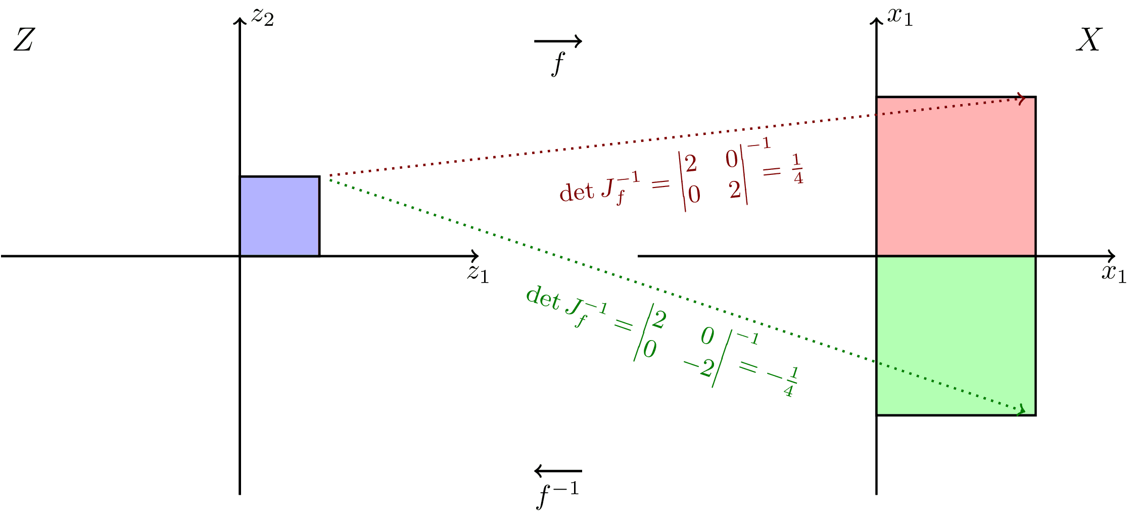
Simple 2d example illustrating the role of the Jacobian determinant in the change of variables formula. Inspired by Ari Seff in https://youtu.be/i7LjDvsLWCg?t=250.
\documentclass[tikz]{standalone}
\usepackage{pgfplots,mathtools}
\pgfplotsset{compat=newest}
\begin{document}
\begin{tikzpicture}[thick]
\draw[->] (-3,0) -- (3,0) node[below] {$z_1$};
\draw[->] (0,-3) -- (0,3) node[right] {$z_2$};
\draw[fill=blue!30] (0,0) rectangle (1,1) node (z1) {};
\node[below right,font=\large] at (-3,3) {$Z$};
\begin{scope}[xshift=4cm]
\draw[->] (-0.3,2.7) -- node[midway,below] {$f$} (0.3,2.7);
\draw[<-] (-0.3,-2.7) -- node[midway,below] {$f^{-1}$} (0.3,-2.7);
\end{scope}
\begin{scope}[xshift=8cm]
\draw[->] (-3,0) -- (3,0) node[below] {$x_1$};
\draw[->] (0,-3) -- (0,3) node[right] {$x_1$};
\draw[fill=red!30] (0,0) rectangle (2,2) node (x1) {};
\draw[fill=green!30] (0,0) rectangle (2,-2) node (x2) {};
\node[below left,font=\large] at (3,3) {$X$};
\end{scope}
\draw[->,dotted,red!50!black] (z1) -- node[midway,below,sloped,font=\small] {$\det J_f^{-1} = \begin{vmatrix} 2 & 0 \\ 0 & 2 \end{vmatrix}^{-1} \mkern-15mu = \frac 1 4$} (x1);
\draw[->,dotted,green!50!black] (z1) -- node[midway,below,sloped,font=\small] {$\det J_f^{-1} = \begin{vmatrix} 2 & 0 \\ 0 & -2 \end{vmatrix}^{-1} \mkern-15mu = -\frac 1 4$} (x2);
\end{tikzpicture}
\end{document}
#import "@preview/cetz:0.3.2": canvas, draw
#set page(width: auto, height: auto, margin: 8pt)
#canvas({
import draw: line, content, rect
let arrow-style = (mark: (end: "stealth", fill: black, scale: 0.5))
let plot-size = 6
let plot-sep = 8
// Helper to draw coordinate axes
let draw-axes(origin, label) = {
// Draw axes
line(
(origin.at(0) - plot-size / 2, origin.at(1)),
(origin.at(0) + plot-size / 2, origin.at(1)),
..arrow-style,
name: label + "-x",
)
line(
(origin.at(0), origin.at(1) - plot-size / 2),
(origin.at(0), origin.at(1) + plot-size / 2),
..arrow-style,
name: label + "-y",
)
// Add axis labels
content((rel: (0, -0.3), to: label + "-x.end"), eval(lower(label) + "_1", mode: "math"), name: label + "-x-label")
content((rel: (0.3, 0), to: label + "-y.end"), eval(lower(label) + "_2", mode: "math"), name: label + "-y-label")
// Add plot label
content(
(origin.at(0) - plot-size / 2, origin.at(1) + plot-size / 2),
text(size: 1.2em)[$#label$],
anchor: "south-west",
name: label + "-title",
)
}
// Draw left plot (Z space)
let z-origin = (0, 0)
draw-axes(z-origin, "Z")
// Draw blue square in Z space
rect(
(z-origin.at(0), z-origin.at(1)),
(z-origin.at(0) + 1, z-origin.at(1) + 1),
fill: blue.transparentize(60%),
name: "z-square",
)
// Draw right plot (X space)
let x-origin = (plot-sep, 0)
draw-axes(x-origin, "X")
// Draw transformed squares in X space
rect(
(x-origin.at(0), x-origin.at(1)),
(x-origin.at(0) + 2, x-origin.at(1) + 2),
fill: red.transparentize(60%),
name: "x-square-1",
)
rect(
(x-origin.at(0), x-origin.at(1)),
(x-origin.at(0) + 2, x-origin.at(1) - 2),
fill: green.transparentize(60%),
name: "x-square-2",
)
// Draw mapping arrows
let mid-x = plot-sep / 2
line(
(mid-x - 0.3, 2.7),
(mid-x + 0.3, 2.7),
..arrow-style,
name: "f-arrow",
)
content("f-arrow.mid", $f$, name: "f-label", anchor: "south", padding: (bottom: 4pt))
line(
(mid-x + 0.3, -2.5),
(mid-x - 0.3, -2.5),
..arrow-style,
name: "f-inv-arrow",
)
content("f-inv-arrow.mid", $f^(-1)$, name: "f-inv-label", anchor: "north", padding: (top: 4pt))
// Draw dotted transformation arrows with determinant labels
line(
"z-square.north-east",
"x-square-1.north-east",
..arrow-style,
stroke: (dash: "dotted", paint: red),
name: "det-arrow-1",
)
content(
(rel: (0.2, -0.2), to: "det-arrow-1.mid"),
[#text(red, $det J_f^(-1) = mat(delim: "|", 2, 0; 0, 2)^(-1) = 1 / 4$)],
anchor: "north",
angle: 5deg,
name: "det-label-1",
)
line(
"z-square.north-east",
"x-square-2.south-east",
..arrow-style,
stroke: (dash: "dotted", paint: green),
name: "det-arrow-2",
)
content(
(rel: (0.2, -0.3), to: "det-arrow-2.mid"),
[#text(green, $det J_f^(-1) = mat(delim: "|", 2, 0; 0, -2)^(-1) = -1 / 4$)],
anchor: "north",
angle: -19deg,
name: "det-label-2",
)
})