Convexity and Jensen’s Inequality
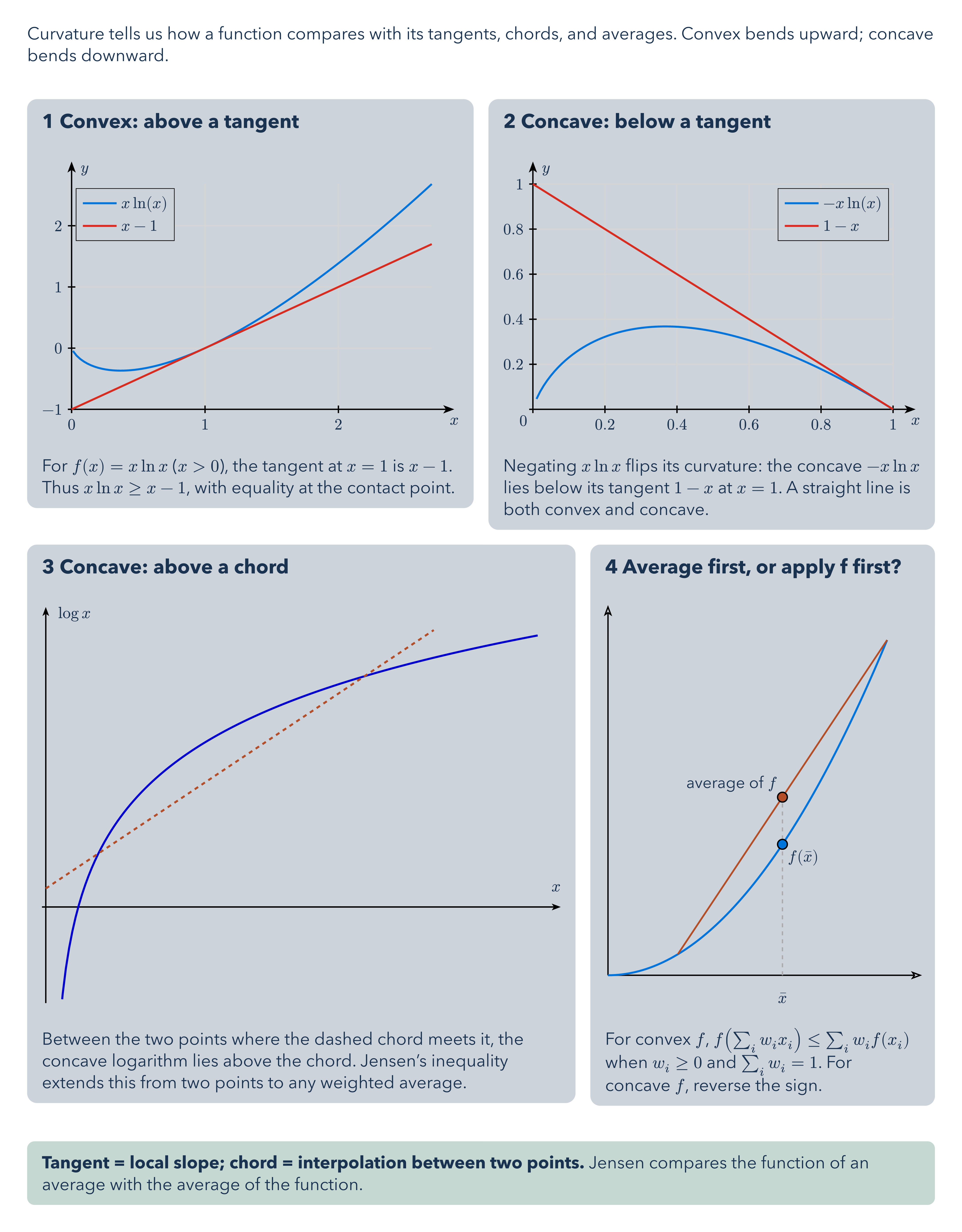
Curvature tells us how a function compares with its tangents, chords, and averages. Convex bends upward; concave bends downward.
Download
Code
#import "@preview/cetz:0.5.3": canvas, draw, vector
#import "@preview/cetz-plot:0.1.4": plot
#let label-size = 12pt
#let paragraph-size = 14pt
#let heading-size = 16pt

#let card_body(title, body, caption) = block(
  width: 100%,
  inset: 12pt,
  radius: 8pt,
  fill: rgb("#cdd3da"),
  breakable: false,
)[
  #text(size: heading-size, weight: "bold", title)
  #v(8pt)
  // Measure unconstrained artwork before scaling, including content wider than its card.
  #layout(size => {
    let artwork = text(size: label-size, body)
    std.scale(size.width / measure(artwork).width * 100%, reflow: true, artwork)
  })
  #v(7pt)
  #text(size: paragraph-size, caption)
]

#let card-grid(columns: 2, ..cards) = layout(size => {
  let rows = cards
    .pos()
    .chunks(columns)
    .map(row => {
      let ratios = row.map(card => {
        let bounds = measure(text(size: label-size, card.at(1)))
        bounds.width / bounds.height
      })
      let available = size.width - 12pt * (row.len() - 1) - 24pt * row.len()
      grid(
        columns: ratios.map(ratio => 24pt + available * ratio / ratios.sum()),
        gutter: 12pt,
        ..row.map(args => card_body(..args)),
      )
    })
  stack(dir: ttb, spacing: 12pt, ..rows)
})

#let takeaway(body) = block(
  width: 100%,
  inset: 12pt,
  radius: 6pt,
  fill: rgb("#c6d8d2"),
  breakable: false,
  text(size: paragraph-size, body),
)

#set page(width: 780pt, height: auto, margin: 22pt, fill: none)
#set text(font: "Avenir Next", size: paragraph-size, fill: rgb("#19324f"))
#set par(leading: 0.55em)

// Tangents and chords, dark enough to stand out on the gray cards in both site themes.
#let tangent-color = rgb("#d62d20")
#let chord-color = rgb("#b24e28")

// Shared frame for the tangent comparisons in panels 1 and 2.
#let comparison-plot(tick-step, legend, curves, ..args) = canvas(length: 1.2cm, {
  let axis-mark = (end: "stealth", fill: black)
  draw.set-style(
    legend: (fill: rgb("#cdd3da")),
    axes: (
      x: (mark: axis-mark, label: (anchor: "north", offset: 0.1)),
      y: (mark: axis-mark, label: (anchor: "north-west", offset: -0.2)),
    ),
  )
  plot.plot(
    size: (8, 5),
    x-label: $x$,
    y-tick-step: tick-step,
    x-tick-step: tick-step,
    x-grid: true,
    y-grid: true,
    legend: legend,
    // Compact legend with a thin border.
    legend-style: (item: (spacing: 0.15), padding: 0.15, stroke: 0.5pt),
    axis-style: "left",
    ..args,
    {
      // Domains start at 0.01 where needed since ln(0) is undefined.
      for (color, domain, samples, label, func) in curves {
        plot.add(
          style: (stroke: color + 1.5pt),
          domain: domain,
          samples: samples,
          label: label,
          func,
        )
      }
    },
  )
})

// === 1  Convex: above a tangent ===
#let figure-0 = comparison-plot(1, "inner-north-west", (
  (blue, (0.01, 2.7), 100, $x ln(x)$, x => x * calc.ln(x)),
  (tangent-color, (0, 2.7), 50, $x-1$, x => x - 1),
))

// === 2  Concave: below a tangent ===
#let figure-1 = comparison-plot(0.2, "inner-north-east", x-min: 0, x-max: 1, (
  (blue, (0.01, 1), 100, $-x ln(x)$, x => -x * calc.ln(x)),
  (tangent-color, (0, 1), 50, $1-x$, x => 1 - x),
))

// === 3  Concave: above a chord ===
#let figure-2 = canvas(length: 1.6cm, {
  let axis-mark = (end: "stealth", fill: black, scale: 0.7)
  draw.set-style(axes: (
    x: (mark: axis-mark, label: (anchor: "south-east", offset: -0.25)),
    y: (mark: axis-mark, label: (anchor: "north-west", offset: -0.2)),
  ))
  plot.plot(
    size: (8, 6),
    x-label: $x$,
    y-label: $log x$,
    y-min: -1,
    x-tick-step: none,
    y-tick-step: none,
    axis-style: "school-book",
    {
      plot.add(
        style: (stroke: rgb(0%, 0%, 80%) + 1.5pt),
        domain: (11, 150),
        samples: 150,
        x => calc.ln(x - 10) - 2,
      )
      // Chord extended past the two points where it meets the curve
      plot.add(
        style: (stroke: (paint: chord-color, thickness: 1.5pt, dash: "dashed")),
        domain: (8, 120),
        x => 0.2 + (3 - 0.2) * (x - 8) / (120 - 8),
      )
    },
  )
})

// === 4  Average first, or apply f first? ===
#let figure-3 = canvas(length: 1.85cm, {
  let curve(x) = 0.3 * x * x
  let chord = (1, 4).map(x => (x, curve(x)))
  let (x-mean, mean-f) = vector.lerp(..chord, 0.5)
  for end in ((4.5, 0), (0, 5.3)) { draw.line((0, 0), end, mark: (end: "stealth")) }
  draw.line(..range(81).map(idx => (idx / 20, curve(idx / 20))), stroke: blue + 1.5pt)
  draw.line(..chord, stroke: chord-color + 1.3pt)
  draw.line((x-mean, 0), (x-mean, mean-f), stroke: (dash: "dashed", paint: gray))
  draw.circle((x-mean, curve(x-mean)), radius: 0.07, fill: blue, name: "f-of-mean")
  draw.circle((x-mean, mean-f), radius: 0.07, fill: chord-color, name: "mean-of-f")
  draw.content((x-mean, -0.25), $macron(x)$, anchor: "north")
  draw.content("f-of-mean", $f(macron(x))$, anchor: "north-west", padding: 4pt)
  draw.content("mean-of-f", [average of $f$], anchor: "south-east", padding: 4pt)
})

Curvature tells us how a function compares with its tangents, chords, and averages. Convex bends upward; concave bends downward.
#v(14pt)
#card-grid(
  (
    [1  Convex: above a tangent],
    figure-0,
    [For $f(x)=x ln x$ ($x>0$), the tangent at $x=1$ is $x-1$. Thus $x ln x >= x-1$, with equality at the contact point.],
  ),
  (
    [2  Concave: below a tangent],
    figure-1,
    [Negating $x ln x$ flips its curvature: the concave $-x ln x$ lies below its tangent $1-x$ at $x=1$. A straight line is both convex and concave.],
  ),
  (
    [3  Concave: above a chord],
    figure-2,
    [Between the two points where the dashed chord meets it, the concave logarithm lies above the chord. Jensen’s inequality extends this from two points to any weighted average.],
  ),
  (
    [4  Average first, or apply f first?],
    figure-3,
    [For convex $f$, $f(sum_i w_i x_i) <= sum_i w_i f(x_i)$ when $w_i >= 0$ and $sum_i w_i=1$. For concave $f$, reverse the sign.],
  ),
)
#v(12pt)
#takeaway[*Tangent = local slope; chord = interpolation between two points.* Jensen compares the function of an average with the average of the function.]