« home

Matsubara Contour 1

physicsquantum field theoryMatsubaracomplex analysisGreen's functionthermal field theorycontour integrationfrequency sumscetztikz

Initial contour C for evaluating Matsubara frequency sums. C runs counterclockwise around the imaginary p₀-axis where the Matsubara frequencies ωₙ = 2πn/β lie, but excludes the poles of the propagator 1/(-p₀² + x²). The integrand includes the Bose-Einstein distribution which has simple poles at all Matsubara frequencies with residue T.
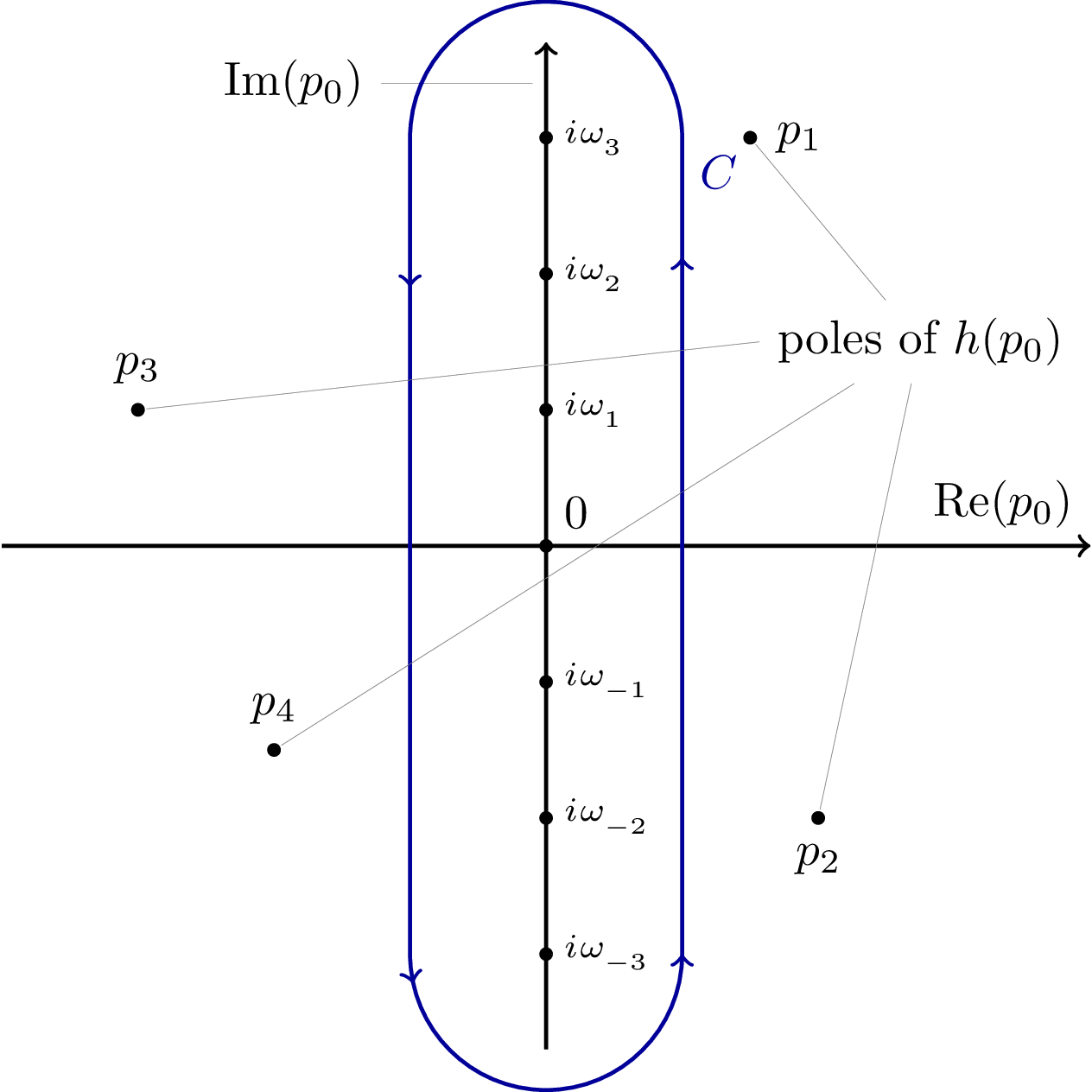

Matsubara Contour 1

  Download

PNGPDFSVG

  Code

  LaTeX

matsubara-contour-1.tex (47 lines)

\documentclass[tikz]{standalone}

\usepackage{mathtools}

\let\Im\relax
\DeclareMathOperator{\Im}{Im}
\let\Re\relax
\DeclareMathOperator{\Re}{Re}

\usetikzlibrary{decorations.markings,positioning}

\providecommand{\poles}{
  \node (poles) at (2.75,1.5) {poles of $h(p_0)$};
  \draw[fill]
  (1.5,3) coordinate [circle,fill,inner sep=1pt,label=right:$p_1$] (p1)
  (2,-2) coordinate [circle,fill,inner sep=1pt,label=below:$p_2$] (p2)
  (-3,1) coordinate [circle,fill,inner sep=1pt,label=above:$p_3$] (p3)
  (-2,-1.5) coordinate [circle,fill,inner sep=1pt,label=above:$p_4$] (p4);
  \draw[ultra thin,gray] (poles) -- (p1) (poles) -- (p2) (poles.west) -- (p3) (poles) -- (p4);
}

\def\xr{3}
\def\yr{3}

\begin{document}
\begin{tikzpicture}[thick]

  % Axes
  \draw [->] (-\xr-1,0) -- (\xr+1,0) node [above left] {$\Re(p_0)$};
  \draw [->] (0,-\yr-0.7) -- (0,\yr+0.7) coordinate [below left = 0.3 and 0.1] (y-axis);
  \node (y-label) at ([xshift=-50]y-axis) {$\Im(p_0)$};
  \draw[ultra thin,gray] (y-axis) -- (y-label);

  % Matsubara frequencies
  \foreach \n in {-\yr,...,-1,1,2,...,\yr}{%
      \draw[fill] (0,\n) circle (1pt) node [right,font=\scriptsize] {$i \mkern1mu \omega_{_{\n}}$};}
  \draw[fill] (0,0) circle (1pt) node [above right] {0};

  % Contour line
  \draw[blue!60!black,decoration={markings,mark=between positions 0 and 1 step 0.28 with \arrow{>}},postaction={decorate}] (1,-\yr) -- (1,\yr) node [below right] {$C$} arc (0:180:1) (-1,\yr) -- (-1,-\yr) arc (180:360:1);

  % Poles of h(p_0)
  \poles

\end{tikzpicture}
\end{document}

  Typst

matsubara-contour-1.typ (119 lines)

#import "@preview/cetz:0.3.4": canvas, draw
#import draw: line, content, circle, arc, set-style

#set page(width: auto, height: auto, margin: 8pt)

// Constants
#let x-range = 3
#let y-range = 3

// Define styles
#let arrow-style = (
  mark: (end: "stealth", fill: black, scale: 0.5),
  stroke: 0.5pt,
)
#let dark-blue = blue.darken(20%)

// Helper function to draw poles
#let draw-poles(poles-label-pos) = {
  // Draw poles label and connecting lines
  content(poles-label-pos, [poles of $h(p_0)$], name: "poles-label")

  // Draw the poles
  circle((1.5, 3), radius: 0.05, fill: black, name: "p1")
  circle((2, -2), radius: 0.05, fill: black, name: "p2")
  circle((-3, 1), radius: 0.05, fill: black, name: "p3")
  circle((-2, -1.5), radius: 0.05, fill: black, name: "p4")

  // Add pole labels
  content("p1", $p_1$, anchor: "west", padding: 2pt)
  content("p2", $p_2$, anchor: "north", padding: 2pt)
  content("p3", $p_3$, anchor: "south", padding: 2pt)
  content("p4", $p_4$, anchor: "north", padding: 2pt)

  // Connect poles to label with thin gray lines
  let stroke = (stroke: (paint: gray, thickness: 0.2pt))
  line("poles-label", "p1", ..stroke)
  line("poles-label", "p2", ..stroke)
  line("poles-label.west", "p3", ..stroke)
  line("poles-label", "p4", ..stroke)
}

#canvas({
  // Draw axes
  line((-x-range - 1, 0), (x-range + 1, 0), ..arrow-style, name: "x-axis")
  content("x-axis.end", $"Re"(p_0)$, anchor: "south-east", padding: 2pt)

  line((0, -y-range - 0.7), (0, y-range + 0.7), ..arrow-style, name: "y-axis")
  content((rel: (-1, 0), to: "y-axis.95%"), $"Im"(p_0)$, name: "y-label", anchor: "south-east", padding: 2pt)
  line("y-axis.98%", "y-label", stroke: (paint: gray, thickness: 0.2pt))

  // Draw Matsubara frequencies
  for n in range(-y-range, y-range + 1) {
    if n != 0 {
      circle((0, n), radius: 0.03, fill: black, name: "freq-" + str(n))
      content(
        "freq-" + str(n),
        $i omega_#text(size: 0.7em)[#n]$,
        anchor: "west",
        padding: (x: 3pt),
      )
    }
  }

  // Draw origin
  circle((0, 0), radius: 0.03, fill: black, name: "origin")
  content("origin", [0], anchor: "south-west", padding: (left: 3pt, bottom: 2pt))

  // Draw contour line
  // Right vertical line
  // Base line with name
  line(
    (1, -y-range - 0.3),
    (1, y-range + 0.3),
    stroke: dark-blue,
    mark: (end: "stealth", scale: 0.5),
    name: "right-line",
  )


  // Top semicircle - positioned to fully enclose the y-axis
  arc(
    (0, y-range + 0.6),
    radius: 1,
    start: 0deg,
    stop: 180deg,
    stroke: dark-blue,
    mark: (end: "stealth", scale: 0.5),
    name: "top-arc",
    anchor: "center",
  )

  // Left vertical line
  line(
    (-1, y-range + 0.3),
    (-1, -y-range - 0.3),
    stroke: dark-blue,
    name: "left-line",
    mark: (end: "stealth", scale: 0.5),
  )

  // Bottom semicircle - positioned to fully enclose the y-axis
  arc(
    (0, -y-range - 0.5),
    radius: 1,
    start: 180deg,
    stop: 360deg,
    stroke: dark-blue,
    mark: (end: "stealth", scale: 0.5),
    name: "bottom-arc",
    anchor: "center",
  )

  // Add contour label
  content("right-line.end", text(fill: dark-blue)[$C$], anchor: "south-west", padding: 2pt)

  // Draw poles
  draw-poles((2.75, 1.5))
})