« home

Matsubara Contour 2

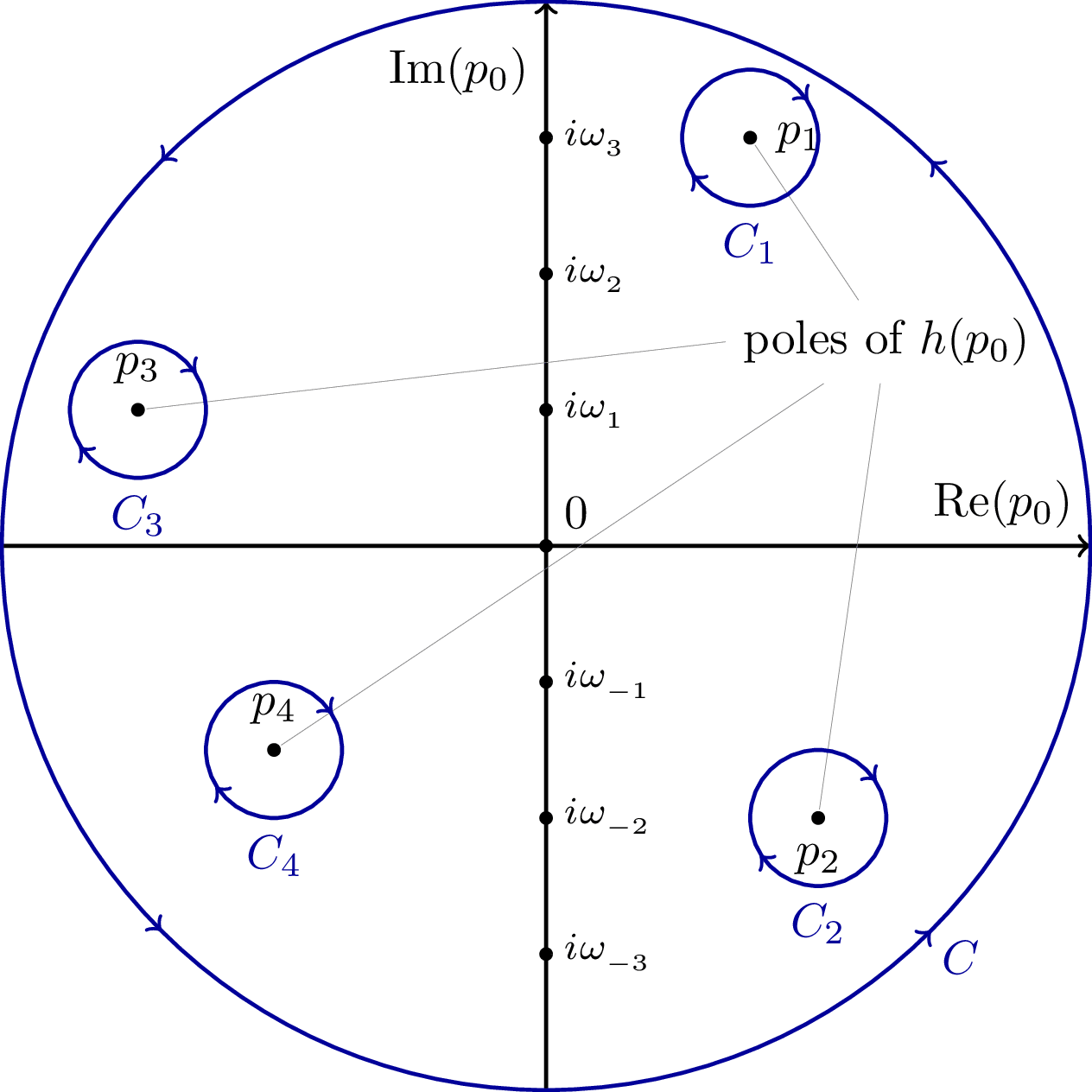
First deformation of the Matsubara contour in https://diagrams.janosh.dev/matsubara-contour-1 where C is expanded into a circle followed by taking the radius to infinity, plus two small clockwise circles C₁ and C₂ around the propagator poles. Since the integrand falls off faster than 1/p₀, the contribution from the large circle vanishes at infinity, leaving only the pole contributions. The small circles around the poles are there to remove again the contribution from the poles that was added by enclosing them in the counterclockwise contour C.

Download

PNG PDF SVG

Code

matsubara-contour-2.tex (55 lines)

\documentclass[tikz]{standalone}

\usepackage{mathtools}

\let\Im\relax
\DeclareMathOperator{\Im}{Im}
\let\Re\relax
\DeclareMathOperator{\Re}{Re}

\usetikzlibrary{decorations.markings,positioning}

\providecommand{\poles}{
  \node (poles) at (2.5,1.5) {poles of $h(p_0)$};
  \draw[fill]
  (1.5,3) coordinate [circle,fill,inner sep=1pt,label=right:$p_1$] (p1)
  (2,-2) coordinate [circle,fill,inner sep=1pt,label=below:$p_2$] (p2)
  (-3,1) coordinate [circle,fill,inner sep=1pt,label=above:$p_3$] (p3)
  (-2,-1.5) coordinate [circle,fill,inner sep=1pt,label=above:$p_4$] (p4);
  \draw[ultra thin,gray] (poles) -- (p1) (poles) -- (p2) (poles.west) -- (p3) (poles) -- (p4);
}

\providecommand{\polecontours}{
  \draw[blue!60!black,decoration={markings,mark=between positions 0.03 and 1.03 step 0.125
    with \arrow{<}},postaction={decorate}] (p1) circle (0.5) node [below=0.5] {$C_1$} (p2)
    circle (0.5) node [below=0.5] {$C_2$} (p3) circle (0.5) node [below=0.5] {$C_3$} (p4)
    circle (0.5) node [below=0.5] {$C_4$};
}

\begin{document}
\begin{tikzpicture}[thick]

  \def\xr{3} \def\yr{3}

  % Axes
  \draw [->] (-\xr-1,0) -- (\xr+1,0) node [above left] {$\Re(p_0)$};
  \draw [->] (0,-\yr-1) -- (0,\yr+1) node [below left=0.2 and 0] {$\Im(p_0)$};

  % Matsubara frequencies
  \foreach \n in {-\yr,...,-1,1,2,...,\yr}{%
      \draw[fill] (0,\n) circle (1pt) node [right,font=\footnotesize] {$i \mkern1mu \omega_{_{\n}}$};}
  \draw[fill] (0,0) circle (1pt) node [above right] {0};

  % Contour line
  \draw[blue!60!black,decoration={markings,mark=between positions 0.125 and 0.875 step 0.25 with \arrow{>}},
    postaction={decorate}] circle (\yr+1) node [below right=0.925*\xr and 0.925*\yr] {$C$};

  % Poles
  \poles

  % Pole contours
  \polecontours

\end{tikzpicture}
\end{document}

matsubara-contour-2.typ (115 lines)

#import "@preview/cetz:0.4.1": canvas, draw
#import draw: arc, circle, content, line, set-style

#set page(width: auto, height: auto, margin: 8pt)

// Constants
#let x-range = 3
#let y-range = 3
#let main-radius = y-range + 1.5
#let pole-radius = 0.5
#let dot-radius = 0.05
#let small-dot-radius = 0.03

// Styles
#let arrow-style = (mark: (end: "stealth", scale: 0.5))
#let dark-blue = blue.darken(20%)
#let marc-style = (symbol: "stealth", fill: dark-blue, scale: 0.5, shorten-to: none)
#let gray-line = (paint: gray, thickness: 0.2pt)

// Helper function to draw poles
#let draw-poles(poles-label-pos) = {
  content(poles-label-pos, [poles of $h(p_0)$], name: "poles-label")

  // Pole positions: (x, y, name, anchor)
  let pole-positions = (
    (1.5, 3, "p1", "west"),
    (2, -2, "p2", "north"),
    (-3, 1, "p3", "south"),
    (-2, -1.5, "p4", "north"),
  )

  for (x, y, name, anchor) in pole-positions {
    circle((x, y), radius: dot-radius, fill: black, name: name)
    content(name, $p_#name.last()$, anchor: anchor, padding: 2pt)

    let connect-point = if name == "p3" { "poles-label.west" } else { "poles-label" }
    line(connect-point, name, stroke: gray-line)
  }
}

// Helper function to draw pole contours
#let draw-pole-contours() = {
  for i in range(1, 5) {
    let name = "p" + str(i)

    arc(
      name,
      radius: pole-radius,
      start: 0deg,
      stop: 360deg,
      stroke: dark-blue,
      mark: (
        end: (
          (pos: 25%, ..marc-style),
          (pos: 75%, ..marc-style),
        ),
      ),
      name: "c" + str(i),
      anchor: "origin",
    )

    content(
      (rel: (0, 0.8), to: "c" + str(i)),
      text(fill: dark-blue)[$C_#i$],
      anchor: "north",
    )
  }
}

#canvas({
  // Draw axes
  line((-main-radius, 0), (main-radius, 0), ..arrow-style, name: "x-axis")
  content("x-axis.end", $"Re"(p_0)$, anchor: "south-east", padding: 2pt)

  line((0, -main-radius), (0, main-radius), ..arrow-style, name: "y-axis")
  content("y-axis.97%", $"Im"(p_0)$, anchor: "north-east", padding: 2pt)

  // Draw Matsubara frequencies
  for n in range(-y-range, y-range + 1) {
    if n != 0 {
      circle((0, n), radius: small-dot-radius, fill: black, name: "freq-" + str(n))
      content("freq-" + str(n), $i omega_#text(size: 0.7em)[#n]$, anchor: "west", padding: (x: 3pt))
    }
  }

  // Draw origin
  circle((0, 0), radius: small-dot-radius, fill: black, name: "origin")
  content("origin", [0], anchor: "south-west", padding: (left: 3pt, bottom: 2pt))

  // Draw main contour
  arc(
    (0, 0),
    radius: main-radius,
    start: 0deg,
    stop: 360deg,
    stroke: dark-blue,
    mark: (
      end: (
        (pos: 12.5%, ..marc-style),
        (pos: 37.5%, ..marc-style),
        (pos: 62.5%, ..marc-style),
        (pos: 87.5%, ..marc-style),
      ),
    ),
    name: "main-contour",
    anchor: "origin",
  )

  content("main-contour.90%", text(fill: dark-blue)[$C$], anchor: "north-west", padding: 2pt)

  // Draw poles and pole contours
  draw-poles((2.5, 1.5))
  draw-pole-contours()
})