DFT MLFF CFF Speed Accuracy Transfer

computational chemistrymaterials sciencedensity functional theorymachine learningforce fieldscetztikz

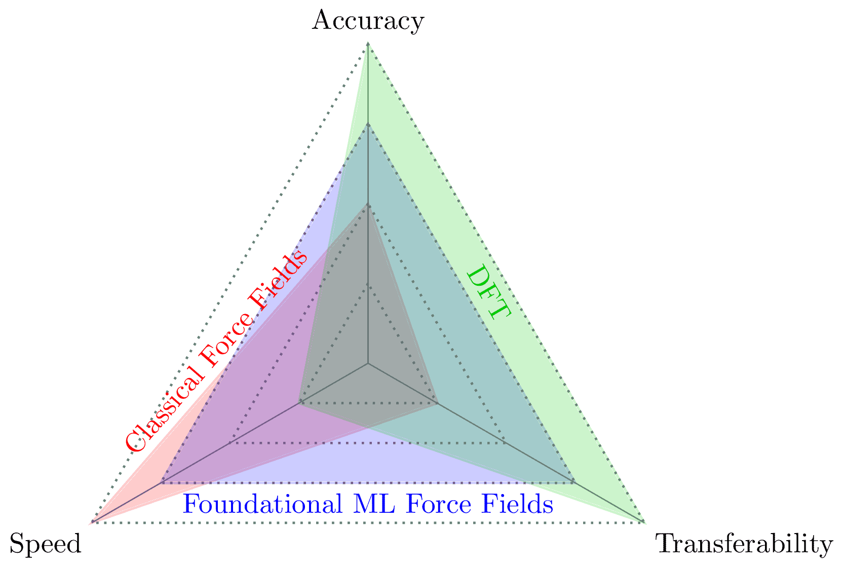
This spider diagram compares three computational chemistry methods: Classical Force Fields, Foundational ML Force Fields, and Density Functional Theory (DFT). The comparison is based on three key attributes:

1. Accuracy: The precision and reliability of the method's predictions.
2. Speed: The computational efficiency and time required for simulations.
3. Generalizability: The ability to be applied across diverse chemical systems and material classes.

• Classical Force Fields (red): Highest speed, medium accuracy, lowest generalizability.
• DFT (green): Highest accuracy and generalizability, but lowest speed.
• Foundational ML Force Fields (blue): Balanced performance across all attributes, positioned between classical methods and DFT.

This diagram shows common trade-offs, highlighting how Foundational ML Force Fields aim to bridge the gap between the speed of classical methods and the accuracy of DFT, while offering improved generalizability over classical force fields.