k-Space

physicssolid state physicscetztikz

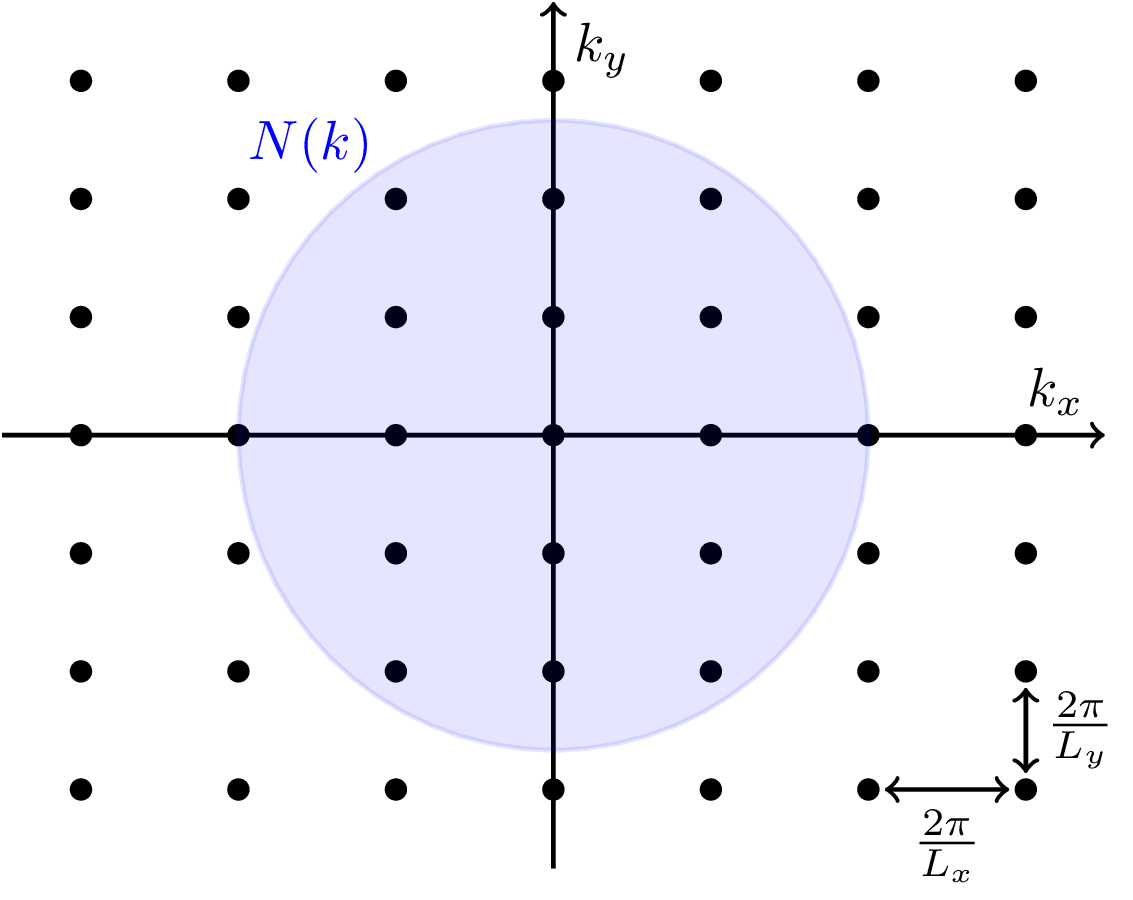
The $k$ -space region of wave vectors up to a given magnitude is a disk of area $\pi k^2$ . The $k$ -space area occupied by a single particle state is

\frac{1}{2} \frac{2 \pi}{L_x} \frac{2 \pi}{L_y} = \frac{2 \pi^2}{A},

where the factor of $\frac{1}{2}$ is due to the spin degeneracy $g_s = 2 s + 1 = 2$ . The number of states with wave vector magnitude smaller than $k$ is

N(k) = \frac{\pi k^2}{2 \pi^2/A} = \frac{A k^2}{2 \pi}.

$k$ -space is used extensively in solid state physics e.g. to visualize the energy bands of a material as a function of electron momentum. In position space, the position-energy dispersion would just be a probability blur.

Download

PNG PDF SVG

Code

LaTeX

k-space.tex (27 lines)

\documentclass[tikz]{standalone}

\begin{document}
\begin{tikzpicture}[thick]

  % Dot grid
  \def\xrange{3}
  \def\yrange{3}
  \def\ratio{3/4}
  \foreach \x in {-\xrange,...,\xrange}
    {\foreach \y in {-\yrange,...,\yrange}
        {\fill (\x,\ratio*\y) circle[radius=2pt];}}

  % Axes
  \draw[->] (-\xrange-1/2,0) -- (\xrange+1/2,0) node[above left] {$k_x$};
  \draw[->] (0,-\ratio*\yrange-1/2) -- (0,\ratio*\yrange+1/2) node[below right] {$k_y$};

  % Lattice spacing
  \draw[<->,shorten >=3,shorten <=3] (\xrange-1,-\ratio*\yrange) -- (\xrange,-\ratio*\yrange) node[midway,below] {$\frac{2 \pi}{L_x}$};
  \draw[<->,shorten >=3,shorten <=3] (\xrange,-\ratio*\yrange) -- (\xrange,-\ratio*\yrange+\ratio) node[midway,right] {$\frac{2 \pi}{L_y}$};

  % Circle
  \draw[blue,fill=blue,fill opacity=0.1] (0,0) circle (2/3*\yrange);
  \node[blue] at (130:2.4) {$N(k)$};
\end{tikzpicture}
\end{document}

Typst

k-space.typ (62 lines)

#import "@preview/cetz:0.3.2": canvas, draw

#set page(width: auto, height: auto, margin: 8pt)

#let x-range = 3
#let y-range = 3
#let ratio = 3 / 4

#canvas({
  // Set up coordinate system
  import draw: circle, content, line

  // Draw blue circle with fill in background
  circle(
    (0, 0),
    radius: 2 / 3 * y-range,
    stroke: blue,
    fill: blue.lighten(80%),
    fill-opacity: 0.2,
    name: "fermi-circle",
  )

  // Draw dot grid
  for x in range(-x-range, x-range + 1) {
    for y in range(-y-range, y-range + 1) {
      circle((x, ratio * y), radius: 2pt, fill: black)
    }
  }

  // Draw axes with arrows
  let arrow-style = (mark: (end: "stealth", fill: black))
  let x-end = (x-range + 0.5, 0)
  let y-end = (0, ratio * y-range + 0.5)

  line((-x-range - 0.5, 0), x-end, ..arrow-style)
  line((0, -ratio * y-range - 0.5), y-end, ..arrow-style, name: "y-axis")

  // Add axis labels
  content(x-end, $k_x$, anchor: "south-west")
  content((rel: (.55, 0), to: "y-axis.end"), $k_y$, anchor: "north-east")

  // Draw lattice spacing indicators with arrows
  let spacing-arrow = (mark: (start: "stealth", end: "stealth", fill: black, scale: .3, offset: 0.1), stroke: 0.7pt)
  let x-start = (x-range - 1, -ratio * y-range)
  let x-end = (x-range, -ratio * y-range)
  let x-mid = ((x-start.at(0) + x-end.at(0)) / 2, x-start.at(1))

  line(x-start, x-end, ..spacing-arrow, name: "x-spacing")
  content("x-spacing.mid", $(2pi) / L_x$, anchor: "north", padding: 0.2)

  let y-start = (x-range, -ratio * y-range)
  let y-end = (x-range, -ratio * y-range + ratio)

  line(y-start, y-end, ..spacing-arrow, name: "y-spacing")
  content("y-spacing.mid", $(2pi) / L_y$, anchor: "west", padding: 0.2)

  // Add N(k) label
  let angle = 130deg
  let label-pos = (calc.cos(angle) * 2.4, calc.sin(angle) * 2.4)
  content(label-pos, text(blue)[$N(k)$])
})