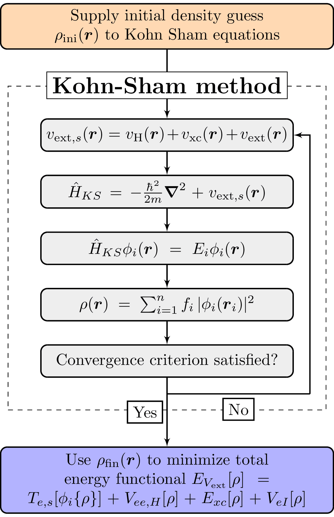
This diagram illustrates the Kohn-Sham cycle in Density Functional Theory (DFT), a computational quantum mechanical modeling method. The process starts with an initial guess for the electron density, which is used to calculate the effective potential. This potential is then used in the Kohn-Sham Hamiltonian, which is solved to obtain the wavefunctions. These wavefunctions are used to compute a new electron density. If convergence criteria are met, the final electron density is used to calculate the total energy functional. If not, the new electron density is used for the next iteration of the cycle.
\documentclass[tikz,svgnames,border={0 2}]{standalone}
\usepackage{mathtools}
\usetikzlibrary{positioning,arrows,fit}
\renewcommand\vec[1]{\boldsymbol{#1}}
\begin{document}
\begin{tikzpicture}[
box/.style={rectangle,draw,fill=DarkGray!20,node distance=1cm,text width=15em,text centered,rounded corners,minimum height=2em,thick},
arrow/.style={draw,-latex',thick},
]
\node [box] (potential) {$v_{\text{ext},s}(\vec r)=v_\text{H}(\vec r) + v_\text{xc}(\vec r) + v_\text{ext}(\vec r)$};
\node [box,below=0.5 of potential] (hamiltonian) {$\hat{H}_{KS}=-\frac{\hbar^2}{2m}\vec{\nabla}^2 + v_{\text{ext},s}(\vec r)$};
\node [box,below=0.5 of hamiltonian] (se) {$\hat{H}_{KS} \phi_i(\vec r)= E_i \phi_i(\vec r)$};
\node [box,below=0.5 of se] (density) {$\rho(\vec r)=\sum_{i=1}^n f_i\,|\phi_i(\vec r_i)|^2$};
\node [box,below=0.5 of density] (criterion) {Convergence criterion satisfied?};
\path
(potential.north west) ++(-1em,1em) coordinate (potential fit)
(criterion.south east) ++(1em,-1em) coordinate (criterion fit);
\node [box,above=1.5 of potential, fill=orange!30, text width=20em] (initial) {Supply initial density guess $\rho_\text{ini}(\vec r)$ to Kohn Sham equations};
\node [box,below=1.5 of criterion, fill=blue!30, text width=20em] (energy) {Use $\rho_\text{fin}(\vec r)$ to minimize total energy functional $E_{V_\text{ext}}[\rho]=T_{e,s}[\phi_i\{\rho\}] + V_{ee,H}[\rho] + E_{xc}[\rho] + V_{eI}[\rho]$};
\path [arrow] (initial) -- (potential);
\path [arrow] (potential) -- (hamiltonian);
\path [arrow] (hamiltonian) -- (se);
\path [arrow] (se) -- (density);
\path [arrow] (density) -- (criterion);
\node [rectangle,draw,dashed,inner sep=1em,fit=(potential fit) (criterion fit)] (enclosure) {};
\node [above=-0.8em of enclosure,anchor=south,draw,outer sep=0pt,fill=white] (enclosure label) {\Large\textbf{Kohn-Sham method}};
\path [arrow] (criterion) -- (energy) node [midway,left=0.1,draw,outer sep=0pt,fill=white] (TextNode) {Yes};
\path [draw,thick] (criterion.south) ++(0em,-1em) -- (criterion fit) node [midway,below=0.1,sloped,draw,outer sep=0pt,fill=white] (TextNode) {No};
\draw [arrow] (criterion fit) |- (potential.east);
\end{tikzpicture}
\end{document}
#import "@preview/cetz:0.3.2": canvas, draw
#set page(width: auto, height: auto, margin: 8pt)
#canvas({
import draw: content, line, rect, on-layer
// Draw dashed enclosure
rect(
(-4, -6),
(4, 3.25),
frame: "rect",
stroke: (dash: "dashed"),
fill: none,
width: 22em,
height: 12em,
name: "enclosure",
radius: 5pt,
)
// Enclosure label
on-layer(
1,
content(
"enclosure.north",
text(weight: "bold", size: 1.2em)[Kohn-Sham method],
frame: "rect",
stroke: black + .5pt,
fill: white,
padding: 3pt,
),
)
let box-style = (
frame: "rect",
stroke: black + .5pt,
fill: rgb("#DCDCDC"),
padding: 8pt,
width: 15em,
)
let arrow-style = (
mark: (end: "stealth", fill: black, scale: .5),
stroke: 1pt,
)
// Initial density box
content(
(rel: (0, 1.25), to: "enclosure.north"),
[Supply initial density guess\ $rho_"init" (arrow(r))$ to Kohn Sham equations],
..box-style,
fill: rgb("#c6aa0c").lighten(60%),
width: 20em,
name: "initial",
padding: (3pt, 2em, 0),
radius: 1em,
)
// Potential box
content(
(rel: (0, -2), to: "initial.south"),
[$v_("ext,s") (arrow(r))=v_H (arrow(r)) + v_"xc" (arrow(r)) + v_"ext" (arrow(r))$],
..box-style,
name: "potential",
)
// Hamiltonian box
content(
(rel: (0, -1.25), to: "potential.south"),
[$hat(H)_"KS"=-frac(planck.reduce^2, 2m)arrow(nabla)^2 + v_("ext,s") (arrow(r))$],
..box-style,
name: "hamiltonian",
)
// Schrödinger equation box
content(
(rel: (0, -1.25), to: "hamiltonian.south"),
[$hat(H)_"KS" phi_i (arrow(r))= E_i phi_i (arrow(r))$],
..box-style,
name: "schrodinger-eq",
)
// Density box
content(
(rel: (0, -1.25), to: "schrodinger-eq.south"),
[$rho (arrow(r))=sum_(i=1)^n f_i |phi_i (arrow(r_i))|^2$],
..box-style,
name: "density",
)
// Convergence criterion box
content(
(rel: (0, -1.25), to: "density.south"),
[Convergence criterion satisfied?],
..box-style,
name: "criterion",
)
// Final energy box
content(
(0, -7.5),
[Use $rho_"final" (arrow(r))$ to minimize total energy functional\
$E_(V_"ext")[rho] = T_(e,s)[phi_i {rho}] + V_(e e,H) [rho] + E_"xc" [rho] + V_"eI" [rho]$],
..box-style,
fill: rgb("#54aef8").lighten(30%),
width: 20em,
name: "energy",
padding: (4pt, 2em, 1pt),
)
// Draw connecting arrows
line("initial", "potential", ..arrow-style)
line("potential", "hamiltonian", ..arrow-style)
line("hamiltonian", "schrodinger-eq", ..arrow-style)
line("schrodinger-eq", "density", ..arrow-style)
line("density", "criterion", ..arrow-style)
line("criterion", "energy", ..arrow-style, name: "converged-yes")
// Yes/No labels
content(
(rel: (0.1, 0), to: "converged-yes.60%"),
[Yes],
frame: "rect",
stroke: none,
anchor: "west",
padding: (3pt, 2pt),
)
// No feedback loop
line(
"criterion",
(3.6, -5),
(3.6, 2),
"potential",
..arrow-style,
name: "converged-no",
)
content(
"converged-no.13%",
[No],
frame: none,
anchor: "north-east",
padding: (-1pt, 2pt),
)
})