« home

RG Flow in Theory Space

physicsquantum-field-theoryrenormalizationrenormalization-groupeffective-actiontheory-spaceuniversalityinfrared-regulatorflow-equationcoupling-constantscetztikz

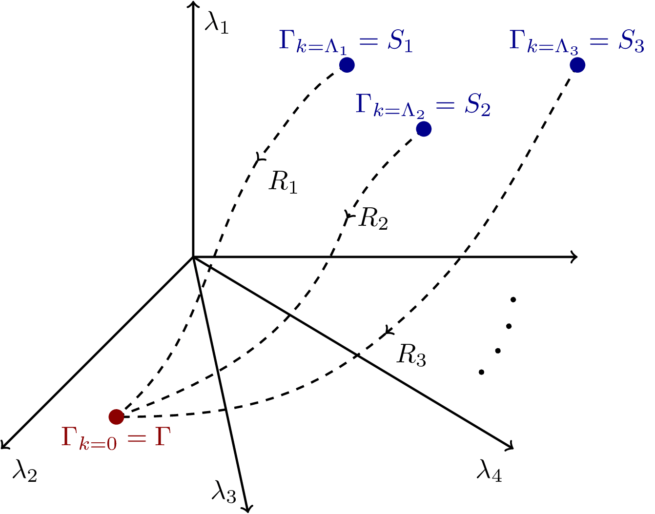
Visualization of renormalization group (RG) flow trajectories in the theory space of all possible coupling constants (λ₁, λ₂, λ₃, λ₄) allowed by symmetries. The diagram shows how different microscopic actions (S₁, S₂, S₃) flow to the same quantum effective action (Γ) through different paths, each corresponding to a different choice of infrared regulator R_k(q). This illustrates the universality of the effective action despite different starting points and regulators.

RG Flow in Theory Space

  Download

PNGPDFSVG

  Code

  LaTeX

rg-flow-in-theory-space.tex (38 lines)

\documentclass[svgnames,tikz]{standalone}

\def\unit{5}

\begin{document}
\begin{tikzpicture}[thick]

  % Coordinates of initial, end and midpoints of transition to complexity
  \coordinate (qea) at (-1/5*\unit,-5/12*\unit); % quantum effective action
  \coordinate (ma1) at (2/5*\unit,1/2*\unit); % microscopic action 1
  \coordinate (ma2) at (3/5*\unit,1/3*\unit); % microscopic action 2
  \coordinate (ma3) at (\unit,1/2*\unit); % microscopic action 3
  \coordinate (r1) at (1/6*\unit,1/4*\unit); % regulator 1
  \coordinate (r2) at (2/5*\unit,1/10*\unit); % regulator 2
  \coordinate (r3) at (1/2*\unit,-1/5*\unit); % regulator 3

  % Coordinate system
  \draw[->] (0,0) -- (0,2/3*\unit) node[below right] (l1) {$\lambda_1$};
  \draw[->] (0,0) -- (-1/2*\unit,-1/2*\unit) node[below right] (l2) {$\lambda_2$};
  \draw[->] (0,0) -- (1/7*\unit,-2/3*\unit) node[above left] (l3) {$\lambda_3$};
  \draw[->] (0,0) -- (5/6*\unit,-1/2*\unit) node[below left] (l4) {$\lambda_4$};
  \draw[->] (0,0) -- (\unit,0);
  \draw[line width=2,line cap=round,dash pattern=on 0pt off 5\pgflinewidth] (3/4*\unit,-3/10*\unit) edge[bend right=20] (5/6*\unit,-1/10*\unit);

  % Flow trajectories
  \draw[dashed] (ma1) edge[->,in=50,out=210] (r1) (r1) node[below right] {$R_1$} to[out=240,in=40] (qea);
  \draw[dashed] (ma2) edge[->,in=60,out=220] (r2) (r2) node[right] {$R_2$} to[out=250,in=20] (qea);
  \draw[dashed] (ma3) edge[->,in=40,out=240] (r3) (r3) node[below right] {$R_3$} to[out=220,in=0] (qea);

  % Initial and end points
  \fill[DarkRed] (qea) circle (0.1) node[below] {$\Gamma_{k=0} = \Gamma$};
  \fill[DarkBlue] (ma1) circle (0.1) node[above] {$\Gamma_{k=\Lambda_1} = S_1$};
  \fill[DarkBlue] (ma2) circle (0.1) node[above] {$\Gamma_{k=\Lambda_2} = S_2$};
  \fill[DarkBlue] (ma3) circle (0.1) node[above] {$\Gamma_{k=\Lambda_3} = S_3$};

\end{tikzpicture}
\end{document}

  Typst

rg-flow-in-theory-space.typ (86 lines)

#import "@preview/cetz:0.3.2": canvas, draw

#set page(width: auto, height: auto, margin: 8pt)

#let unit = 5

#canvas({
  import draw: line, content, circle, hobby

  let arrow-style = (mark: (end: "stealth", fill: black, scale: 0.5))

  // Define coordinates
  let qea = (-0.225 * unit, -5 / 12 * unit) // quantum effective action
  let ma1 = (0.4 * unit, 0.5 * unit) // microscopic action 1
  let ma2 = (0.6 * unit, 0.33 * unit) // microscopic action 2
  let ma3 = (unit, 0.5 * unit) // microscopic action 3
  let r1 = (0.17 * unit, 0.25 * unit) // regulator 1
  let r2 = (0.4 * unit, 0.1 * unit) // regulator 2
  let r3 = (0.5 * unit, -0.2 * unit) // regulator 3

  // Draw coordinate system
  line((0, 0), (0, 0.67 * unit), ..arrow-style, name: "lambda_1")
  content("lambda_1.end", $lambda_1$, anchor: "south")

  line((0, 0), (-0.5 * unit, -0.5 * unit), ..arrow-style, name: "lambda_2")
  content("lambda_2.end", $lambda_2$, anchor: "north-east")

  line((0, 0), (0.14 * unit, -0.67 * unit), ..arrow-style, name: "lambda_3")
  content("lambda_3.end", $lambda_3$, anchor: "north")

  line((0, 0), (0.83 * unit, -0.5 * unit), ..arrow-style, name: "lambda_4")
  content("lambda_4.end", $lambda_4$, anchor: "north-west")

  line((0, 0), (unit, 0), ..arrow-style)

  // Draw dotted line segment
  hobby(
    (0.75 * unit, -0.3 * unit),
    (0.82 * unit, -0.2 * unit),
    (0.83 * unit, -0.1 * unit),
    stroke: (dash: "loosely-dotted", thickness: 1.5pt),
  )

  // Draw flow trajectories using hobby curves
  hobby(
    ma1,
    r1,
    (0, -.8),
    qea,
    stroke: (dash: "dashed"),
  )
  content(r1, $R_1$, anchor: "north-west")

  hobby(
    ma2,
    r2,
    (0, -1.7),
    qea,
    stroke: (dash: "dashed"),
  )
  content(r2, $R_2$, anchor: "north-west")

  hobby(
    ma3,
    r3,
    qea,
    stroke: (dash: "dashed"),
  )
  content(r3, $R_3$, anchor: "north-west")

  // Draw points and labels
  let dark-red = rgb("8B0000")
  circle(qea, radius: 0.1, fill: dark-red, stroke: none)
  content((rel: (0, -0.2), to: qea), text(fill: dark-red)[$Gamma_(k=0) = Gamma$], anchor: "north")

  let dark-blue = rgb("00008B")
  circle(ma1, radius: 0.1, fill: dark-blue, stroke: none)
  content((rel: (0, 0.2), to: ma1), text(fill: dark-blue)[$Gamma_(k=Lambda_1) = S_1$], anchor: "south")

  circle(ma2, radius: 0.1, fill: dark-blue, stroke: none)
  content((rel: (0, 0.2), to: ma2), text(fill: dark-blue)[$Gamma_(k=Lambda_2) = S_2$], anchor: "south")

  circle(ma3, radius: 0.1, fill: dark-blue, stroke: none)
  content((rel: (0, 0.2), to: ma3), text(fill: dark-blue)[$Gamma_(k=Lambda_3) = S_3$], anchor: "south")
})